
Anatomy of a Climate Model
Nov 16, 2020
Editor's Note: In June, we published Part I of a series of articles that describe AIR's groundbreaking new framework for climate risk modeling, which will enable our suite of atmospheric peril models to capture climate signals at all scales, from local correlations to global teleconnections. Part II, published in September, discussed the relationship between weather and climate, and how Earth’s climate system gives rise to extreme weather events.
For this third article, we are honored to have Professor Henk Dijkstra as a co-author. Dr. Dijkstra is an internationally renowned scientist, expert in the field of dynamical systems methods to problems in climate modeling, climate variability, and climate change. He is the author of several books and numerous articles covering different aspects of climate dynamics and climate change in the biosphere, hydrosphere, and atmosphere. Dr. Dijkstra is a member of an international team of leading scientists supporting AIR in our effort to build a new generation of catastrophe models capable of providing a global view of all weather-related perils in a manner efficient from a technological point of view.
In this article, Part III of the series, we explore numerical climate models; how these models further our understanding of these relationships; and how these relationships may be changing as Earth's surface temperatures continue to rise. We also touch briefly on the limitations of numerical climate models, a topic that will be further explored in Part IV.
As discussed in Part II, planetary-scale atmospheric and oceanic motions are the drivers of local weather extremes—the very extremes that result in large financial losses. To understand the dynamics between weather and climate, and how they may be altered as a result of climate change, scientists employ climate models, which numerically simulate planetary circulations and their interactions at various scales.
The first mathematical models of the atmosphere were developed decades ago. In 1904 physicist and meteorologist Vilhelm Bjerknes proposed that the principles of fluid dynamics could be used to predict atmospheric flows and hence the weather. In 1950 the first successful numerical weather prediction was made by a team under the leadership of the mathematician and physicist John von Neumann. The first 24-hour forecast took nearly an entire day to compute.
Today, a range of numerical models is available for the forecasting of weather and climate phenomena, each of which has been developed for specific forecasting or research purposes; they can differ in terms of spatial domain and resolution as well as the time period for which the forecast is valid. Numerical models are based on primitive equations, which include terms for the conservation of mass; a form of the Navier-Stokes equations governing fluid flow; and thermodynamic terms. Examples of numerical models include numerical weather prediction (NWP) models and global (and regional) general circulation models (GCM).
NWP models are atmospheric models that currently have a horizontal resolution of about 10 km; they may be regional or global in scope. With these models, only simulations over a short period of time (typically 14 days) can be performed. Because of the chaotic nature of atmospheric flows, the forecasting capability decreases dramatically beyond a two-week period. Furthermore, to produce a reasonably accurate forecast, using accurate initial conditions are important. These initial conditions represent a “known state” of the atmosphere and are constructed using observation data available through data-assimilation techniques.
To account for uncertainty in the initial conditions, many simulations (typically 50) with different initial conditions are performed to create a statistical forecasting product (Figure 1). From this product, the probability of specific extreme events, such as severe thunderstorms, hurricanes, heat waves, and extreme precipitation, can be assessed. The forecasts that result from this process allow people, governments, and organizations to not only plan daily activities but also prepare for disasters, up to 14 days in advance.
 Henk Dijkstra, Ph.D.
Professor of Dynamical Oceanography, Institute for Marine and Atmospheric research, Utrecht; and Director, Centre for Complex Systems Studies, Department of Physics, Utrecht University
 Boyko Dodov, Ph.D.
Vice President and Director, AIR Worldwide
The Promise of General Circulation Models
High-resolution NWP models are used primarily for weather forecasting. They cannot be used to make climate predictions on longer (seasonal to decadal) time scales with accuracy, not only because their resolution would require vast computing resources to do so, but also because they are not coupled with an ocean model. As we learned from Part II, weather patterns can be influenced by dynamics that involve both the atmosphere and ocean. The El Niño-Southern Oscillation (ENSO) is just one example of an atmospheric-oceanic phenomenon that affects weather—including tropical cyclone activity—worldwide. Enter the general circulation model, or GCM.
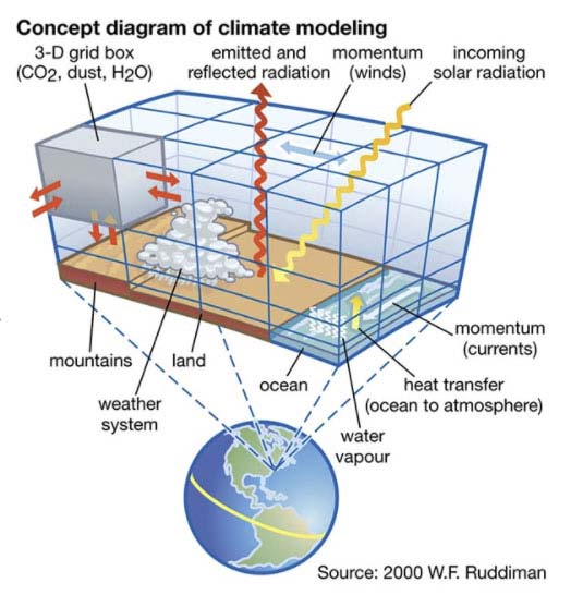
GCMs attempt to simulate a coarse-grained approximation of Earth’s entire climate system. The most complex and resource-intensive component of a GCM is the atmospheric module, which uses the primitive equations to simulate the evolution of wind direction, wind speed, temperature, humidity, and atmospheric pressure, hereafter denoted as U, V, T, Q, and P, respectively. GCMs also include equations describing the oceanic circulation: how it transports heat and how the ocean exchanges heat and moisture with the atmosphere. Another important component is a land surface model that describes how vegetation, soil, and snow or ice cover exchange energy and moisture with the atmosphere. And yet another component captures the interactions between the atmosphere and the cryosphere (sea and land ice).
To solve the equations on a computer, GCMs divide the atmosphere, oceans, and land into a three-dimensional (3-D) grid (Figure 2). The equations are then numerically evaluated in each grid cell at successive time steps throughout the simulation period. The number of cells in the grid determines the model’s resolution, or granularity. Each grid cell is characterized by the average value of each variable; therefore each cell effectively has a uniform velocity, temperature, etc.
While the most recent, state-of-the-art atmospheric GCMs might have a horizontal resolution of 25 km, the more typical GCM used for seasonal predictions and El Niño forecasting, for example, will have a horizontal resolution of about 100 km; a vertical resolution of about 1 km; and a time-stepping resolution of about 10 to 30 minutes. The horizontal resolution of the atmospheric component of most GCMs included in the World Climate Research Programme's Coupled Model Intercomparison Project (CMIP) is ~100 km, or 10 times coarser/lower than current NWP models. If they were to operate at a more granular/higher resolution, GCMs would represent some processes with more realism; however, the computational time required to do the calculations would increase substantially. For example, a doubling of resolution requires about 10 times more computing power because the time step must be halved; not only are there four times as many grid points to evaluate, but twice as many time steps are also required for the model to get to the same point in the future. Thus for most of the world’s climate modeling centers, modeling a spatial resolution beyond 0.5 degrees (60 km at the equator) is not practicably feasible at present. The choice of model resolution is driven both by the available computer resources and by what physical, chemical, and biological processes are relevant to the model’s unique purpose, which dictates the length and number of simulations to be conducted.
The part of a GCM that solves the primitive equations for U, V, T, Q, and P is called the dynamical core. Climate processes represented by this dynamical core are referred to as being “resolved” by the model. But with uniform values within grid cells available, the typical GCM is too coarse to solve important small-scale processes, including those that govern the extreme weather events of interest to catastrophe modelers, such as thunderstorms, tornadoes, and extreme rainfall events. Such “unresolved” sub-grid processes are therefore parameterized—and the parameterization formulas employed (which vary with the scientist or scientists involved) introduce uncertainty and potential bias. The issue of uncertainty and bias and how to reduce it in the context of catastrophe modeling will be discussed in further detail in Part IV.
GCMs and Climate Projections
Today, GCMs (sometimes combined with higher-resolution regional climate models for region-specific results) are providing forecasts of Earth’s climate up to the end of this century. Uncertainty in the initial conditions doesn’t play an important role here because the effect of model error dominates. Therefore, in addition to ensembles with different initial conditions, ensembles with different model parameters are used to evaluate the model error. Because many different GCMs are used, each with their specific biases, a multi-model analysis also provides a measure of uncertainty in the projections.
It’s important to note that, despite the inherent model errors and biases, GCMs still do a reasonably good job of simulating general climate behavior: storms develop and move in realistic ways; temperatures change according to time of day and day of year in realistic ways; and precipitation falls where and when it should—generally. But the details—how intense storms will become, exactly where they will track or stall, and how heavy the precipitation will be—are not captured well enough to satisfy the catastrophe modeler.
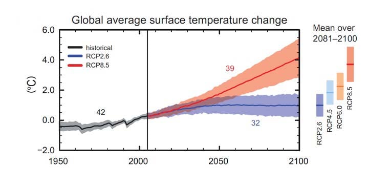
In addition to model error, a major source of uncertainty when making climate projections over decades is the radiative forcing (the difference between energy in the form of sunlight absorbed by Earth and the energy radiated, or reflected, back into space) induced by anthropogenic greenhouse gas (GHG) emissions. GHG emissions depend largely on the usage of fossil fuels and thus human behavior. To cope with this uncertainty, the climate research community makes use of a suite of several emissions scenarios called Representative Concentration Pathways, or RCPs. Each RCP represents a potential trajectory of atmospheric GHG concentrations over the coming decades, culminating in a specific excess radiative forcing at the year 2100. The RCP8.5 scenario, for example, assumes high and growing emissions that will lead to an 8.5 W/m2 extra radiative forcing in the year 2100 and an average increase in surface temperatures of between 2.6°C and 4.8°C (at the 90% confidence level).
In the CMIP5 (CMIP Phase 5) projects undertaken in support of the Intergovernmental Panel on Climate Change (IPCC), the participating GCMs perform a set of predefined simulations resulting in an ensemble of climate projections. Each model first performs a century-long simulation under preindustrial initial conditions, which consist of prescribed solar forcing, aerosol forcing, and greenhouse gas forcing as of the year 1850. This serves as a control simulation. At the end of the control simulation, a so-called historical simulation is performed from 1850 to (usually) 2005. Next, the simulation is continued under one of the RCP scenarios.
For many models, more than one simulation is performed by starting the historical simulation from a different year than the one for the start of the control simulation. The reason being that, although the atmosphere responds quickly to various forcing conditions, the ocean takes much longer; thus at different years in the control simulation the ocean will be very different. These efforts then lead to probabilistic projections of, for example, the global mean surface temperature up to the year 2100 (Figure 3) for the different RCPs. Note that due to the uncertainties in both models and forcing, the behavior of the actual climate system can deviate from these results substantially, and even be outside the estimated range of possibilities illustrated by the shading in Figure 3.
In the realm of climate science, the principal goal of GCMs has been to forecast changes in average surface (land and ocean) temperatures. To determine whether the occurrence of extreme events will change over the next decades, large ensembles are needed, as such events are by definition rare. Several studies indicate that the probability distribution of extreme events will change as Earth’s climate continues to warm. In the case of annual maximum temperature, for example, in many continental-scale regions the mean shifts to higher temperature and the amplitude of the positive tail of the distribution increases. Probabilities of occurrences of these extremes and the return period of specific amplitude extremes can be calculated from these results.
The Next Frontier: Overcoming Uncertainty and Bias in GCMs for Use in Catastrophe Models
GCMs are powerful tools built for purpose; however, none has been built with the catastrophe modeler in mind. While the IPCC’s periodic Assessment Reports speculate on the likely increase in precipitation, for example, they are sparing in their commentary around the frequency and severity (and regional variation) of convective storms, tropical cyclones, and wildfires.
The central question then is: What confidence do we have in the model results as they relate to unobserved extreme events? While we must accept the uncertainties around greenhouse gas forcing, which will always have to be handled by scenarios, there are ways that we can reduce the spectrum of uncertainties and biases that arises through model error and parameterization. The next article in our series will explore these issues and point to AIR’s solution for overcoming them.