
Interconnectedness today works in many directions—as a force that triggers risk contagion, for example, but also as a force motivating intellectual and scientific collaboration. In the biological sciences, the study of quantitative interconnectedness can be traced back to the 1970s. At that time Professor Robert May had already begun to promote the idea that seemingly chaotic growth and expressions of various risk factors are deeply interdependent.
At times of shock and extreme events, such interdependence serves to magnify the force and impact of risk factors through contagion and network effect, which in normal operating circumstances may not manifest. Since the 2007–2012 credit and sovereign debt crisis, concepts such as network contagion have been transferred from ecology and epidemiology to describe the propagation of systemic financial and insurance risks within the wider economy and society.
Such intellectual property transfers equip practitioners in the insurance and financial industries to be able to define the market value of risk, which in its broadest concept can be defined as the sum of technical value of risk and market sentiment. As modelers and product developers, our core promise to the industry is to provide the most realistic, modern, and accurate view of the technical value of risk. To unify modern methodologies and best industry practices we have incorporated these lessons learned and first principles in the 2021–22 development of our Next Generation Models.
This blog explores how some first principles of mathematical ecology and biology sciences are relevant to financial risk management today. It also defines some dependencies and inter-operability between key (re)insurance portfolio risk metrics that are widely used by practitioners today in their risk management and capital reserving functions.
Enforced or Natural Accumulations of SCR
Undoubtedly there is enforced or assumed sub-additivity in the standard solvency capital reserve formula (SCR) Equation 1 in Figure 1. The SCR metric by line of business, geo-admin unit, and risk factor is in principle a value-at-risk metric. By definition value-at-risk metrics are not guaranteed to be sub-additive—or to be super-additive.
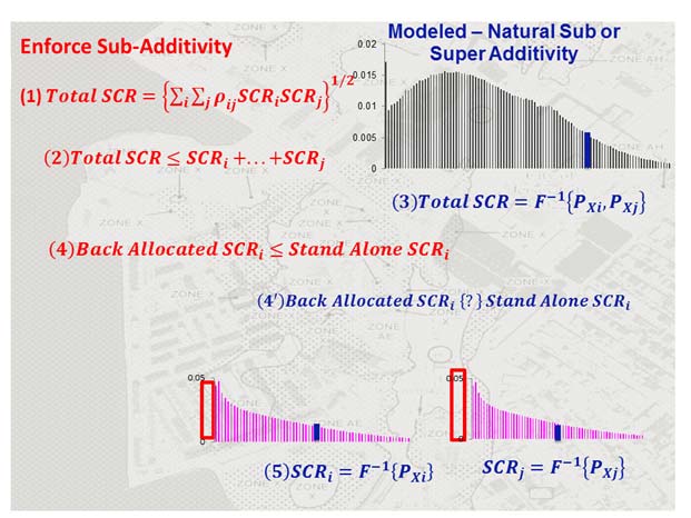
The relationship between the accumulated portfolio total SCR and the sum of the portfolio component SCR(s) is empirical and theoretically unknown. Still the standard SCR formula guarantees, or rather enforces, sub-additive accumulation, as defined in Equation 2 in Figure 1. If the risk factors are guaranteed to be either independent or very well-known and measured dependent on physical and economic laws—such as geography, (in)dependence across extreme events, and financial diversification—this should be a safe and acceptable assumption.
Still the practitioner view will not agree with the purist mathematician’s view of the modeled world. The latter will require the construction of a multivariate probabilistic distribution or copula, as defined in Equation 3 in Figure 1 from the marginal distributions of all risk factors provided in Equations 5 in Figure 1. Only from the combined aggregate distribution of all risk factors in the portfolio could one then coherently measure the portfolio SCR. And because it is a value-at-risk type metric, it is not guaranteed to be neither sub- nor super-additive; it is a purely empirical and scenario-based relationship.
The standard formula also guarantees that a back-allocated single risk factor SCR (i.e., component SCR) is less than the same stand-alone SCR, as provided in Equation 4 in Figure 1. Economists will immediately see the benefits of diversification and market scale. The true coherent back-allocated SCR from the joint distribution is not that easy to compute, however, and it is certainly not guaranteed to behave predictably versus the predictable and enforced stand-alone SCR.
Capital Back-Allocation by the Covariance Principle
For portfolios of risks with a high degree of clustering and concentration, risk and capital metric (back)allocation is best accomplished and most widely done in industry by the covariance principle described in Figure 2 with four equations. Less well used is the second attribute of this principle, which accounts for dispersion and diversification. The critical technical task for application of this principle is to decompose the total (re)insurance portfolio covariance into single risk-to-total components and define the back-allocation ratio as shown in Equation 1 and Equation 2 in Figure 2.
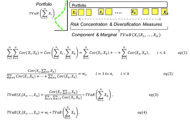
Deriving the expression for back-allocation now becomes quite trivial and is formalized in Equation 3 and Equation 4 in Figure 2. The mechanics are written in the context of tail value at risk (TVaR), and will also apply to value at risk (VaR) and SCR.
Component and Marginal TVaR Converge
Estimating component and marginal TVaR(s) is one of the most computationally intensive tasks in the capital allocation process. These two-risk metrics are actually convergent, which we show with a four-equation proof in Figure 3. Standalone TVaR is defined as a risk metric computed for each risk factor or portfolio component independently from the rest of the book of business. We define component TVaR as the metric statistically back-allocated from the total portfolio TVaR. With a well-known and widely used back-allocation methodology it contains covariance risk, as the Portfolio TVaR takes into account inter-risk dependencies.
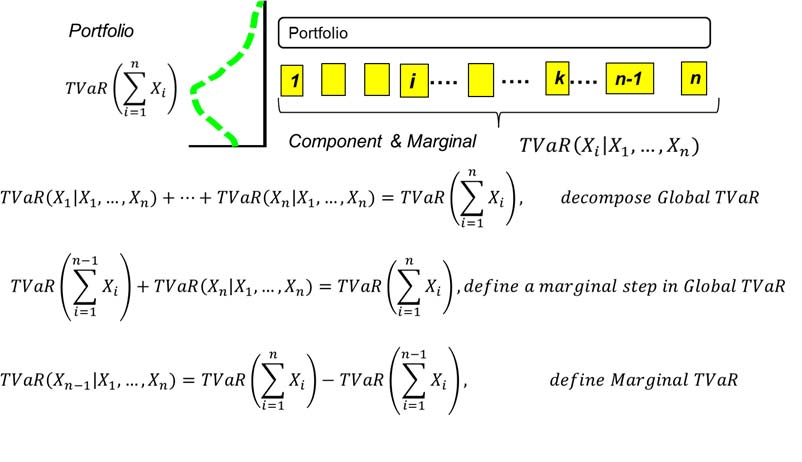
In Equation 1 in Figure 3 we back-allocate the total portfolio metric using a stand-alone TVaR ratio to the portfolio risk components—i.e., this gives us our component TVaR(s). These are cumulative and sub-additive as proved in Equation 2. Then in Equation 3 we show that the sum of the marginal risk metrics leads to the total portfolio metric. Rearranging in Equation 4, we derive the marginal TVaR, which is also our component TVaR. Effectively we have two metrics converging, derived with only a single computation. In other words, once we have our stand-alone metrics and total portfolio TVaR, the marginal metric becomes purely analytical.
Practice in the Science of Risk Ranking
All participants in the (re)insurance value chain practice risk ranking—including the insured(s). The methodologies vary from theoretical to empirical and to numerical simulations, to historical best practices, and such that are reliant on expert knowledge. Regardless of the underlying theory, one still needs a robust ranking metric. In this section I’ll attempt to show that choosing a ranking metric can actually be done in a systematic manner. Let’s look at three metrics—pure technical premium, variance, and tail-value-at-risk (TVaR)—and their fitness for purpose as a preferred risk ranking metric.
Firstly, all three metrics allow the ability to back-allocate from the top portfolio metric to its risk components, such as lines of business and single risks, and reversely accumulate single and component risk metrics to lines and business units. All three metrics satisfy these criteria. They are either additive or sub-additive, which is sufficiently good for the practitioner.
Secondly comes the appreciation of ruin scenarios in addition to appreciation of volatility. Pure technical premium and variance—the latter being contained in the former—emphasize knowledge of volatility while TVaR emphasizes information from worst-case scenarios, which may lead to severe difficulties for the firm or even to its insolvency.
A third requirement may be the ability to perform risk ranking at business unit (BU) level. The relative riskiness of a BU or a single line is already implied in the accumulated total premium of the unit. The risk of the expected outcome and its variance is already priced into the total accumulated BU premium. Premium and variance become unsuitable as risk ranking measures because the insurer already prices their relativity; however, the relative riskiness of TVaR by BU is not accounted for in premium pricing. Practically it is not accounted for in capital allocation in many cases as the preferred metric for capital allocation is value-at-risk (VaR).
A fourth requirement is that the metric provide stability and robustness. All three metrics are affected by marginal impact to the book of business because of dependencies among risks. A change to the profile of one risk factor affects the change of the risk profile of the whole portfolio both in terms of most likely outcomes and tail outcomes.
Lastly, for a practical risk ranking metric these four criteria are best met by TVaR. The relative riskiness of other metrics is already implicit in the price of insurance risk, thereby making them risk neutral; by using them for ranking purposes, such analytics do not bring additional informational value to the underwriter or risk manager. As TVaR sits outside the definition of the price of (re)insurance risk, it brings new information value to the ranking process.
The Epidemiology of Risk Accumulation
The global financial system, defined as including the insurance and reinsurance firms, can be viewed as one large organism where firms of various sizes are interconnected and interdependent. The larger the firm, in terms of assets and risk exposure, the more complex connections it bears to other firms and to the system as a whole.

Larger scale means disproportionately larger risk. This is a thesis, inspired by the biological sciences, in opposition to the traditional financial theory of diversification and economies of scale, which states that with size and distributed exposures come the benefits of stability and durability.
Biological theory, however, from its first principles states that the larger the unit in a biological system or organism the more interconnected and interdependent it becomes on other units and on its living environment as a whole. This makes it more complex and harder to survive a systemic shock. Simple organisms adapt and survive crisis and shock better than large and complex ones.
Should these principles apply to the financial system and its firms, then it would be scale—not diversification—that defines risk management and capital reserving. Large scale requires disproportionately larger reserves and disproportionately more intense precautions by executive management. Mathematicians call this effect super-additivity; however, diversification, de-concentration and sub-additivity remain proved principles of classical financial theory. Yet on a systemic level, it is critical to continuously re-appreciate and revisit which principles dominate and define risk management and capital reserving practices.
Editor’s note: This blog was created from a paper presented by Ivelin Zvezdov at the National Bureau of Economic Research and International Risk Management Society Conference 2018-2019.
Read the AIR Current article “Next Generation Modeling: Loss Accumulation”