
I recently read Nassim Taleb’s book The Black Swan: The Impact of the Highly Improbable (I know … late to the party). There are good lessons to be learned from it, and it had me looking back at my student days and how much I hated the “bag of marbles” way of teaching probability.
The bag of marbles analogy—if you are not familiar with it—asks questions such as, “If you have a bag of marbles with 10 black and 5 white marbles and take one at random, what’s the likelihood of it being white?” It is, of course, a very simplistic example. My point, as highlighted by The Black Swan, is that probability concepts tend to be presented as part of an ideal world that rarely exists. I eventually managed to find my way around such theorems, but I always had to resort to some sort of trick to make them more real so that I could understand them.
I can’t be the only one to have made sense of theorems this way, but what The Black Swan showed me is that perhaps resorting to these types of tricks was the right way to go all along. Understanding theorems and probability from a theoretical point of view is one thing, but applying those tools to the real world is a different matter altogether—which is why I don’t like the “bag of marbles.”
In this post I will show two simple examples to give you a fresh perspective on how we understand probability. They are simple but not simplistic, and will hopefully shed light on the following two questions: “What does reality say about our models?” and “How do we understand the probability of an event?”
What does reality say about our models?
Let me start by telling you about a shrewd character, who relies on empirical experience, and his academic counterpart. Presented with a coin that is fair—with an equal probability of it coming up heads or tails—both are posed the same question: “If I flip it 99 times and get heads each time, what’s the probability of getting tails on my next throw?”
The academic jumps to the mathematically correct answer: 50%. The shrewd character, on the other hand, has a more practical approach: “No more than 1%, of course,” he says, based on the fact that the odds of the coin coming up heads 99 times in a row are so low that “the coin gotta be loaded. It can't be a fair game."
Maybe he is right, maybe he is not.
The truth is, however, perhaps neither is.
The academic was too quick to accept the premise of a fair coin, despite what empirical evidence suggested, and the shrewd character was eager to rely solely on what he saw. Both failed to use both pieces of information in conjunction—the initial assumption and the observation—to evaluate whether the empirical evidence corroborated or disproved the “model” (I could go a bit further on Bayesian inference, but let’s leave that for another day).
Both were victims of their own biases and preconceptions, which brings me to my next point:
How do we understand the probability of an event?
You and I will likely sympathize with the shrewd character in the sense that the likelihood of the coin coming heads 99 times in a row is indeed extremely low—1 in 299, to be more precise. To give you an idea of how small a probability this is, 299 is 6 with 29 zeros, give or take. We’re talking about a probability that is practically zero for all intents and purposes. However, it is important to note that this is the exact same probability of getting any other sequence of heads and tails.
Let’s bring this to an example we can actually get our heads around: What is the probability of seeing each of the following two sequences in 10 coin flips?
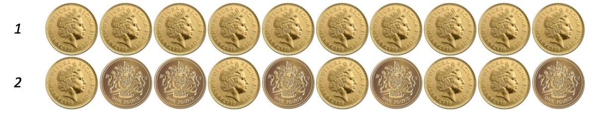
One might be tempted to say sequence 2 is more likely, but both outcomes have exactly the same probability of being observed. Because the likelihood of coming heads or tails is the same (i.e., 50%), any possible sequence has the same likelihood: 1 in 210 (or 1 in 1,024).
You may want to think about it this way: The probability of seeing sequence 1 is the probability of seeing heads on the first throw multiplied by the probability of seeing heads in the second throw, and so on; and the probability of seeing sequence 2 is the probability of seeing heads in the first throw multiplied by the probability of seeing tails in the second throw, and so on. Both are computed exactly the same way:
50% x 50% x 50% x 50% x 50% x 50% x 50% x 50% x 50% x 50% = 0.098% (or 1 in 1,024)
So why were we (well, at least I was) so quick to assume that the second sequence is more likely than the first? The problem was that, in our heads, we were not comparing the probability of seeing the first sequence against that of observing exactly the second one. We were comparing the likelihood of sequence 1 against a sequence different from that. In fact, against any sequence different from that.
Sequence 2 seems much more likely because it resembles one of many outcomes we would expect, which is why we attribute much more likelihood to it. The probability of an outcome different from sequence 1 is 1,022 in 1,024 (1,022 corresponding to all the possible 1,024 sequences minus the one with all heads and the one with all tails). This corresponds to 99.8%, practically an inevitability, whereas the likelihood of observing exactly sequence 2 is 0.098%.
What can we learn from this story? The two key takeaways are:
- Beware of your own biases and preconceptions regarding a given model and how reality conforms to it
- Don’t let your mind jump to conclusions as to what an “event” is. Your assumptions may have far from negligible consequences.
These are very important warnings in the world of catastrophe modeling, and since I started this article by harping on the importance of transporting theoretical concepts to reality, I’ll end with the following two examples of how you may find yourself victim to such preconceptions.
Catastrophe models are fantastic tools, but what you give is what you get. For instance, if you make a mistake when you characterize your portfolio (for example, coding exposed assets as “light metal” when in fact they are well designed steel structures) you’ll end up with a very precise result that happens to be precisely wrong. It’s mathematically correct, but it does not conform to reality.
A good example of the second takeaway is how we perceive the phenomenon of event clustering. One might be tempted to see a cluster in a year with several events. However, that year alone tells us very little in this respect. Whether clustering exists or not can only be determined when looking at the frequency pattern in many years. Clustering isn’t many events in a year (that’s frequency), it is where the pattern of the number of events per year is different from a Poisson distribution.
The moral of the story is: never trust the results blindly.
Read “The Aesthetics of Probability” for a discussion about making probability easier to envision