A New Framework for Global Climate Simulation, Purpose-Built for the Catastrophe Modeling Community

Editor's Note: Part IV of our Climate Change series took a closer look at how catastrophe modelers have employed climate models to develop large catalogs of potential extreme events and why the limitations of these models in a catastrophe modeling context have motivated AIR to develop a new framework for climate risk modeling. For this fifth and penultimate article in our series, we lay out the framework for overcoming those limitations and arriving at a solution purpose-built for the catastrophe modeling community.

We are honored to have Professor Themistoklis Sapsis as a co-author of this article. Dr. Sapsis is Associate Professor of Mechanical and Ocean Engineering at MIT. He received a diploma in Ocean Engineering from Technical University of Athens, Greece, and a Ph.D. in Mechanical and Ocean Engineering from MIT. Before becoming a member of the faculty at MIT, he was appointed Research Scientist at the Courant Institute of Mathematical Sciences at New York University. He has also been visiting faculty at ETH-Zurich. Prof. Sapsis’ work lies on the interface of nonlinear dynamical systems, probabilistic modeling, and machine-learning methods. A particular emphasis of his work is the formulation of mathematical methods for the prediction and statistical quantification of extreme events in complex engineering, physical, and environmental systems.

This article introduces a new framework for modeling atmospheric perils—one that allows for the creation of very large, global catalogs that capture all types of dependencies, from global teleconnections to local correlations across all weather-related perils, across all regions. Importantly, the new framework will allow us to answer not only today's climate questions, but tomorrow's as well.

Reanalysis as Benchmark

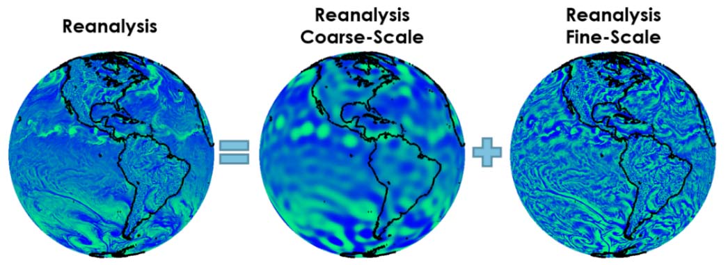
Atmospheric reanalysis is a long-standing and ongoing project that uses data assimilation techniques to combine all available instrumental observations of past weather with simulations from numerical models to produce a complete and statistically, physically, and dynamically consistent recreation of the history of Earth’s weather and climate. The reanalysis used in the development of AIR’s framework is the ECMWF’s ERA5, a fifth-generation reanalysis product covering the period from 1950 to the present, at a 0.25⁰ spatial resolution and hourly timestep.

AIR has divided the data into several frequency (or, conversely, wavelength) bands, from fine to coarse scale. The schematic in Figure 2 shows two such bands. These bands provide benchmarks for machine learning to determine the dependencies between the coarse and fine scales, as well as for debiasing our coarse-scale GCM. Note that reanalysis data is characterized by many hundreds of variables. Our goal is to resolve the full complexity of atmospheric circulation only in the context of catastrophe modeling, so only those weather and climate descriptors relevant to catastrophe models need to be considered, making the task more focused.

Step 1: Debiasing the Coarse-Scale Climate Model (GCM) Output

As just noted and discussed in some detail in Part IV, the currently available state-of-the-art (high resolution) GCMs are not a good fit for the future of catastrophe modeling, both because of their biases and their computational cost. When run at a coarse resolution, however, the output from a state-of-the-art climate model is comparable to the output from a coarse one with simplified physics. A coarse and simple climate model has the advantage of speed; thus, we can use it to generate large catalogs of physically based atmospheric flow very quickly.

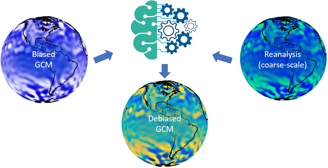
But given that these catalogs will be biased, our framework first requires us to debias the GCM output to ensure that we’re producing realistic frequencies of atmospheric blocking, the polar jet, and other dynamical phenomena, as discussed in Part II. Otherwise, we cannot count on getting an unbiased representation of the frequency of stalled hurricanes like Sandy and Harvey, prolonged droughts like those ahead of the 2019-2020 Australia bushfires, or atmospheric rivers like the one that resulted in the Great Flood of 1862 that devastated Oregon, Nevada, and California. To do that we need to debias the climate model output by benchmarking it to “reality” in the form of the coarse-scale component of the reanalysis data (thus pairing the resolutions of the two data sets).

It’s worth pointing out that this first step in our approach is a research project in itself, involving the application of cutting-edge machine learning techniques to perform the complex and high-dimensional mapping illustrated in Figure 3. This debiasing corrects both the local intensities of the model output parameters, as well as the patterns of these parameters evolving over time—that is, the atmospheric dynamics. By thus correcting the atmospheric dynamics of our simple climate model, we can get storm tracks, for example, and their frequency right. At the end, we have a fast-running, albeit still coarse, GCM without statistical and dynamical biases in the model output.

Step 2: Learning the Behavior of Fine-Scale Features as a Function of the Coarse-Scale Ones

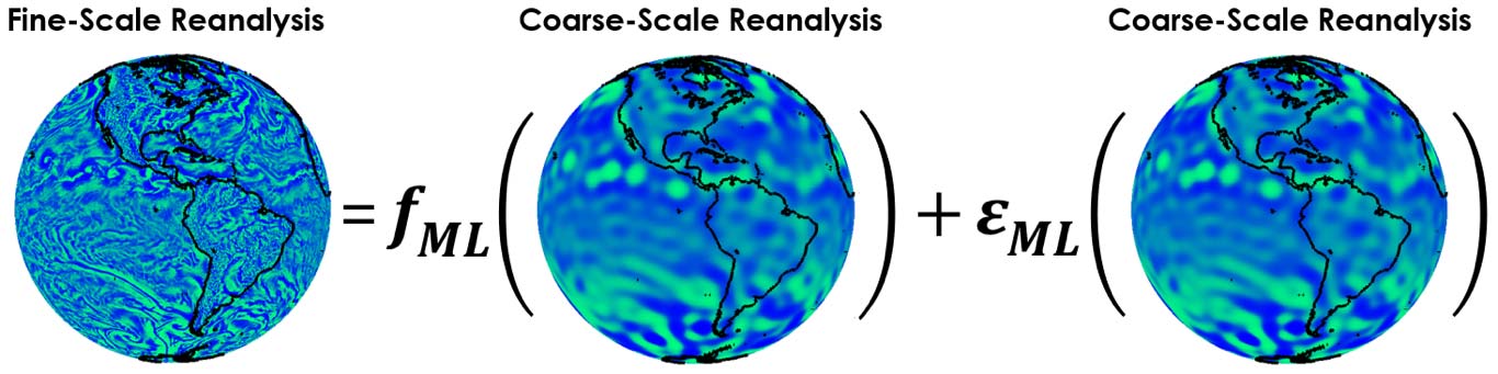
The second step in the process achieves our goal of effectively replicating the output of a state-of-the-art GCM without actually employing one. That is, we reproduce fine-scale atmospheric circulations as a function of coarse-scale ones. We describe how we achieved this through our deep-learning algorithm in the following paragraphs.

The reanalysis data split into coarse and fine frequency bands acted as our training data, which was fed into the probabilistic machine learning algorithm. The algorithm learned two sets of rules from these data: (1) The primary set of rules governed the learning of deterministic dependencies—that is, the expectations of the fine-scale variables as functions of the coarse-scale ones; (2) the second set of rules is where we machine learned the statistics of the residuals of fine-scale variables, after the first set of rules was applied. These sets of rules are denoted as (1) ƒ_ML and (2) ε_ML in Figure 4; they are the end product of Step 2 in our framework.

This probabilistic machine-learning framework presents many exciting opportunities for using these functions in catastrophe modeling applications. We can employ them to quantify hazard uncertainty and create multiple versions of each stochastic event. In the context of historical and real-time events, the probabilistic ML framework can also be used to more faithfully calibrate the modeled hazard footprints to observations through data assimilation. While there are any number of additional benefits that can result from this research, our focus in the next section is on combining steps 1 and 2 to build global, multi-peril catalogs.

Combining Steps 1 and 2 into a Robust and Efficient Global Simulation of Atmospheric Dynamics

Recall that in Step 1 we debiased the output of our coarse-scale GCM. Step 2 gave us two sets of rules for simulating fine-scale dynamics from the coarse-scale GCM output, thus achieving the results of a state-of-the-art GCM but at low cost. Figure 5 illustrates how putting the solutions from Step 1 and Step 2 together allows us to efficiently simulate large global physics-driven catalogs with realistic dynamics and robust statistics at all scales.

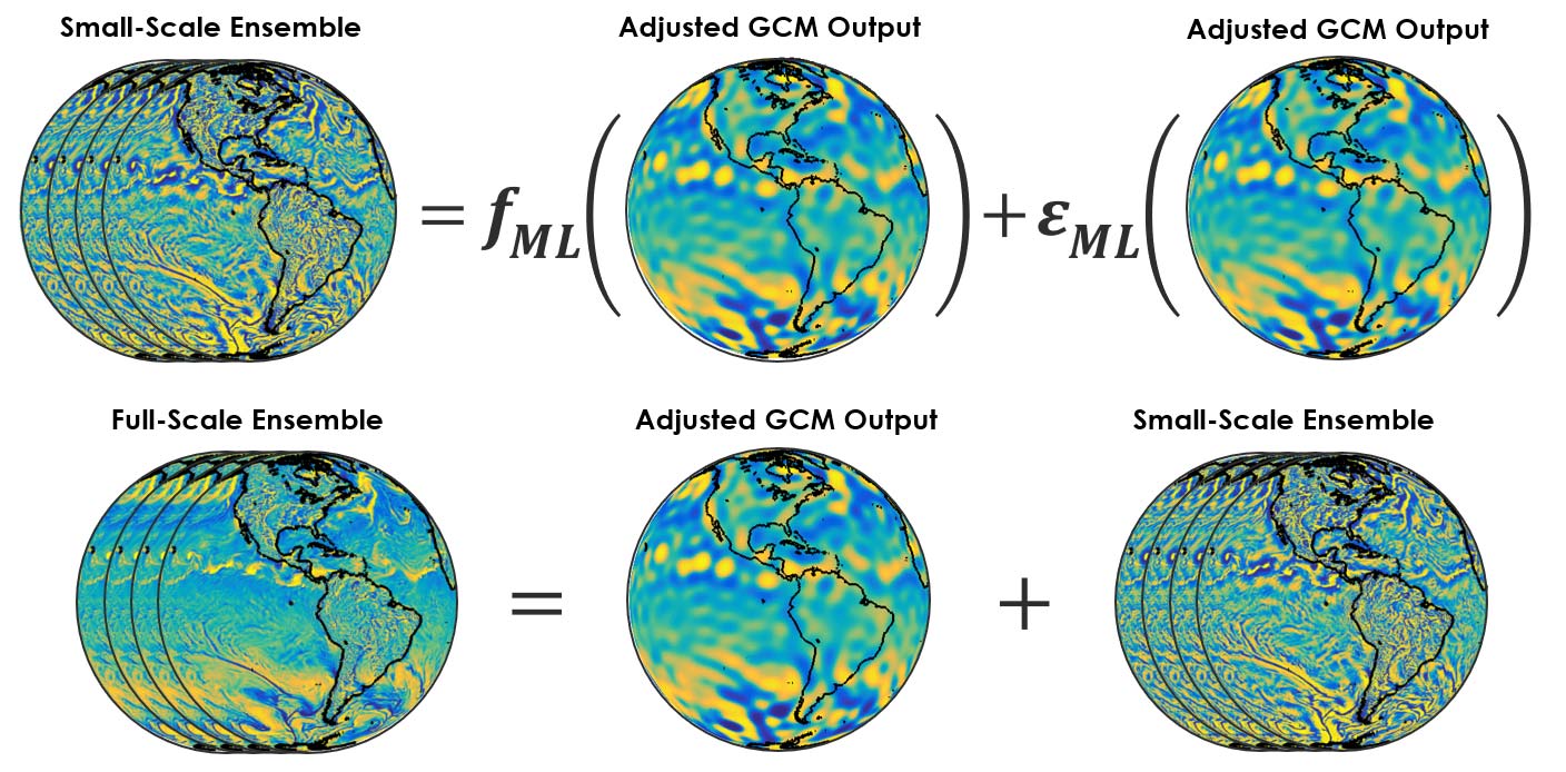
To do that, we plug the adjusted large-scale variables from the simple climate model output from Step 1 into the machine-learned sets of rules obtained from Step 2 to simulate ensembles of fine-scale time series. We then add the large-scale and the ensemble small-scale variables to obtain the final full-scale catalog.

Next Step: Fundamentally Change How Weather and Climate Are Simulated

The most sophisticated atmospheric peril models available to the insurance industry currently rely on perturbations of reanalysis data that are restricted to fine scales. This is because perturbing the large scales will make the event footprints unrealistic. Perturbing only the small scales, however, results in large-scale patterns that too closely resemble historical events, which are then repeated many times over in a stochastic catalog. The same would happen to parametric models that use large-scale reanalysis data for conditioning—that is, we may never see large-scale patterns capable of producing events far more severe than Hurricane Harvey, even though we know they are physically possible. Without the ability to explicitly simulate the large-scale patterns, we will never understand the probability of occurrence of atmospheric dynamics that give rise to the most extreme events—more extreme than historical events and in locations other than we’ve observed.

The new framework under development at AIR will address these issues and will fundamentally change the way weather and climate are simulated in the industry. Those tasked with managing risk will have access to large, robust global catalogs that capture all types of dependencies—from local correlations to global teleconnections and across all atmospheric perils, including tropical and extratropical cyclones, floods, severe thunderstorms, and droughts.

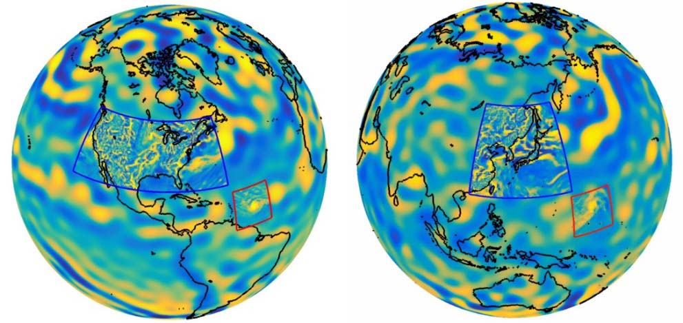
The coarse model output will have the correct frequency and magnitude statistics of large-scale phenomena, such as blocking, cyclogenesis, and Rossby waves, as well as the fine-scale signatures of tropical cyclones and convective storms. We can use the framework such that it can move around such a signature to simulate tropical cyclone wind and precipitation. Alternatively, we can train our algorithm with regional reanalysis data and add small scale detail to a specific region, such as the U.S., or Japan (Figure 6).

Finally, we can leverage the stochastic nature of our catalogs for efficient catalog versioning, where the versions can be conditioned on climate change or climate index oscillations. The next article, the last in our series, will describe how our new modeling framework can be used to provide insights into the potential impacts of climate change on the locations, frequencies, and intensities of extreme events.