
Modeling Fundamentals: Understanding Tectonic Movement and How It Sheds Light on Seismic Risk
Nov 12, 2018
Editor's Note: Kinematic modeling techniques use a physical approach to understanding earthquake risk, effectively augmenting the sparse available historical data. AIR Seismologist Dr. Bingming Shen-Tu explains what kinematic modeling is and provides real-world examples in South America, China, Japan, and New Zealand of how effective it is.
A World in Motion
"Everything moves, nothing stands still," said the Greek philosopher Heraclitus 2,500 years ago. He was speaking philosophically, of course, not seismically. He would not have understood how literally true his statement is. In fact, almost no one did until 50 years ago. The modern understanding of plate tectonics—the realization that the earth's land masses, rigid plates that make up the earth's crust both above the oceans and below them, are in constant motion and tension with respect to each other—was confirmed only in the 1960s.
The movement of these plates, however, is slow. For example, the subduction of the Nazca plate under the South American plate is just 70–80 millimeters per year. But the movement is relentless. After eons, the result is the configuration of the Earth's surface as we know it today. The subduction zone off the west coast of South America has led to uplift of the Andes mountain range and has produced some of the largest earthquakes in the world, including the largest earthquake on record, the 1960 M9.5 earthquake in southern Chile.
Despite the ages-long timescale of plate motion, it nonetheless impacts the otherwise fleeting experience of human beings: through earthquakes, tsunamis, volcanoes, and their effects. In the tectonic play of irresistible forces, eventually something gives, or breaks, or moves aside. The Earth quakes.
Modeling Earthquake Occurrence
Earthquake models are used to help anticipate and mitigate such disasters by providing estimates of where, how big, and how often earthquakes are likely to occur in the future. After a major rupture, such as the 500-km long rupture within the Nazca subduction zone beneath central Chile that triggered the M8.8 Maule earthquake on February 27, 2010, the likelihood of another large earthquake on that fault is reduced. Forecasting large earthquakes on subduction zones is difficult, however, because rupture areas often overlap and rupture magnitude can vary considerably. This produces a very complex pattern of overlapping fault segments that may be fully locked, partially locked, or relaxed, and thus capable of producing earthquakes of different magnitudes with different probabilities.
An even bigger challenge is the scarcity of information on past earthquakes. While South America has a long history of seismic activity, featuring some of the strongest earthquakes on the planet, some other regions of the world do not. They can experience earthquakes where none had ever been recorded, where no fault had been mapped, and in an area thought to be seismically inactive.
Large earthquakes are thought to rupture most commonly along active faults at regular time intervals, and the magnitude of each recurring rupture is thought to be roughly the same—that is, a magnitude that is "characteristic" of that fault. This regularity results from the unremitting pressure produced by the movement of the tectonic plates, which remains essentially the same over time. Thus, after a fault ruptures, the amount of time it will take for sufficient energy to build up before the next rupture will be about the same for each recurrence.
In the case of some earthquakes the build-up period could have been 400 or 500 years—or longer, but a record was never made or was lost. This has been the experience in many regions of the world: incomplete records, inadequate information about important earthquake characteristics (magnitude, length of the fault, movement along the fault, etc.), or no records at all. Indeed, the largest earthquakes usually have the longest recurrence intervals—more than 500 or even thousands of years—to before the invention of writing. The lack of sufficient historical records for such earthquakes was one of the main reasons seismologists were unaware of the potential occurrence of some recent earthquakes, such as the 2008 Wenchuan earthquake in China and the 2010 Tohoku earthquake in Japan.
Augmenting the historical record, researchers can also make use of paleoseismic information—data about pre-historic earthquakes derived from such activities as fault trenching. However, the paleoseismic record is considerably sparser than the historical record.
Kinematic Modeling—A Physical Approach
Fortunately, data helpful to overcoming the limitations of historical and paleoseismic data have become available in recent years through the application of new technology. The movement by an entire land mass of just millimeters per year may be too little and too slow for human beings to perceive, but for instruments on satellites, it is not. By using the Global Positioning System (GPS) and other geodetic tools (world-surveying systems, usually from orbit) to precisely monitor and probe specific locations on the Earth's surface over time, the movement of different parts of land masses relative to each other can be measured.
Enter kinematic modeling, a daunting term that describes a relatively simple concept. Kinematics is the branch of classical mechanics that describes the motion of objects. Indeed, plate tectonics—the large-scale movement of the earth's lithosphere—is a kinematic model, albeit a coarse-resolution one.
 Bingming Shen-Tu, Ph.D.
Vice President, Director, Earthquake Hazard Research
Edited by Sara Gambrill, CEEM
The article:
• Estimating the location and frequency of earthquakes that have long return periods is centrally important to seismic risk assessment, yet the historical and paleoseismic records are spotty at best and provide limited guidance; kinematic modeling offers a physically based approach to understanding earthquake occurrence.
• In developing an earthquake model for a region, AIR seismologists must estimate where potential future earthquakes are likely to occur, as well as how often they will occur and how big they will be.
• The results from the kinematic model can be used to constrain the long-term regional seismicity model, and when they are combined with the historical and paleoseismic data, can be used to estimate seismic slip accumulation on a fault and thus provide valuable information about constraint on the time dependency of earthquake rupture probability.
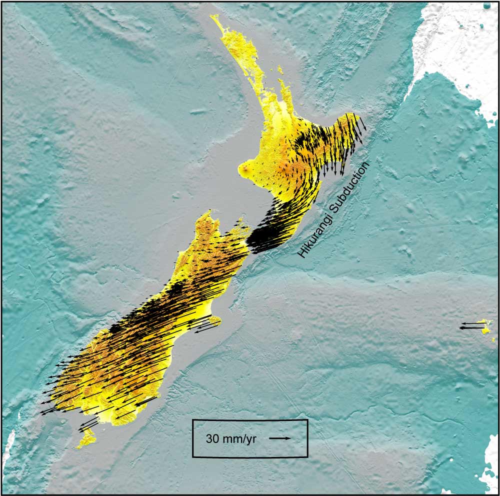
At a considerably finer resolution, Figure 1 shows the relative velocities of the Earth's crust in New Zealand as determined from GPS surveys. The length of the arrows is indicative of the speed of motion (relative to the benchmark 30 mm/year arrow shown in the legend), while the orientation of the arrows indicates direction of movement. Any change in length or direction of the arrows is indicative of ongoing crustal deformation in the area. As can be seen, the deformations in this region are quite complex.
Through kinematic modeling, these physical measurements can be used to augment the historical record and greatly enhance our understanding of earthquake occurrence within the crustal layer (within the top 20-50 km).
Alternative Strategies, Same Objective
There are two widely used approaches to kinematic modeling. The first is based on the assumption that the seismic actors are rigid fault blocks and that crustal deformation takes place only along block (or, on a larger scale, plate) boundaries. Thus, its implementation is simple and direct—but it relies on assumptions about where the faults (the block boundaries) are located. When the assumed fault locations deviate from actual locations, the model can produce unrealistic results. Kinematic block models also necessarily simplify the dynamics of regional tectonics. The main advantage of this approach is that it estimates fault slip rates and other parameters that can be directly used in seismicity model development. For subduction zones, a block model can estimate the rate of seismic slip accumulation along the fault, which can provide important information on the amount of seismic energy that has accumulated or is accumulating along the subduction zone.
The other strategy assumes that the crust behaves like a viscous fluid and models that behavior along a continuum. This approach requires making fewer assumptions. For example, estimates of fault locations are not needed, although when such information is available it can be used—along with historical catalog data, fault geometry, and slip rates—as additional, powerful input to make the kinematic model more reliable. Indeed, results from the block-based technique can also be incorporated.
AIR seismologists and researchers use both approaches to assist in the development of a catalog of shallow, or crustal earthquakes for our earthquake models. Although GPS survey data has been used in seismic hazard studies for more than two decades, kinematic model results of GPS data have generally been used indirectly in the development of regional hazard models. This situation may start to change as the USGS has recently used the deformation rates from kinematic models directly to constrain the seismicity rate in the latest earthquake model for California—the Uniform California Earthquake Rupture Forecast Model, Version 3 (UCERF3).
Applying Kinematic Modeling in AIR Earthquake Models
Using the GPS data as primary input, but incorporating all other available data as well, AIR seismologists define and overlay a three-dimensional grid on the model domain. Each of the cells of varying size that make up the grid is defined to capture a crustal volume that exhibits a relatively homogeneous deformation pattern. By applying a mathematical procedure known as inversion, GPS data, plate motion velocities, and other available data are converted into a strain rate for each cell. Strain rates capture how quickly the Earth’s shallow crust is being deformed and therefore how quickly seismic energy is accumulating within the shallow layer of the crust where most of the damaging earthquakes originate.
Several types of data, such as active fault, historical earthquake, and geodetic data, can be used to calculate the strain rates in the grid cells. These different data sets are all indicative of deformation in the seismogenic crust during various time scales: active faults are indicative of deformation that has occurred during the last few thousand to few million years; earthquakes are indicative of the crustal deformation rate in the last few hundred or few thousand years; and GPS data measures the deformation rate in the last few decades. Each data set has its limitations and uncertainties. A kinematic model can use one or more of the above data sets to develop a self-consistent regional deformation field that matches any of the observed strain rates or velocity data in a region within their bounds of uncertainty while also satisfying certain boundary conditions such as plate motions.
New Zealand and Kinematic Modeling
In the case of New Zealand, for example, Figure 2 demonstrates that the continuous deformation field obtained from the kinematic modeling of the GPS data in Figure 1—fault information— and Pacific-Australia plate motion velocity depicts higher strain rates (orange and red) in most areas where seismic activity has been high in the last 100 to 130 years. Most larger historical earthquakes have occurred in the Hikurangi subduction zone, the Puysegur subduction zone, the Marlborough Shear Zone (MSZ), and the Taupo Volcanic Zone (TVZ), where the GPS data–constrained kinematic model shows higher strain rates.
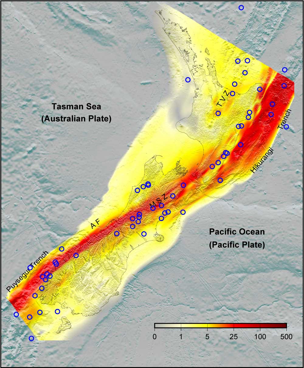
The deformation field obtained from GPS data represents the total tectonic strain rates within the crust, which represent how fast the crust has been deforming during the last two to three decades. Not all strain accumulated in the crust will be released by earthquakes. Fault creeping can release strain due to tectonic forces along weak fault surfaces. On the other hand, large earthquakes can release strain rates in a large volume of crust along two sides of the fault surface. Hence the strain rates accumulated off the fault plane will be released as transient elastic strain, rather than by earthquakes off the fault. The block model can provide additional information about fault creeping and transient deformation of major faults.
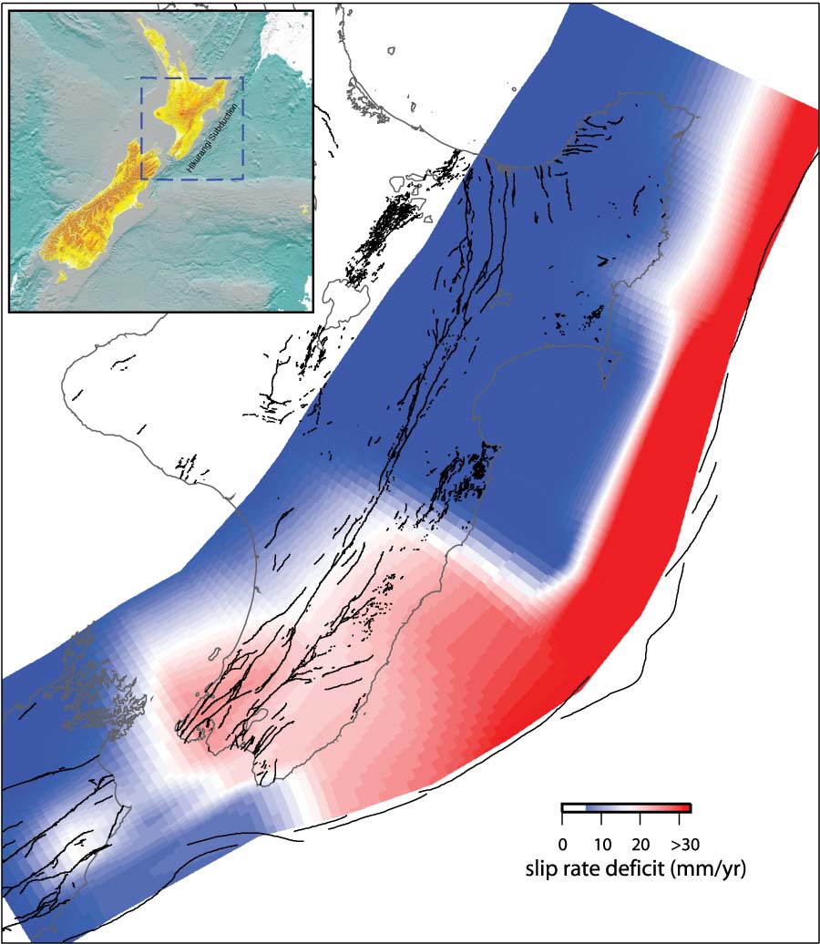
Figure 3 shows the deformation rates along the Hikurangi subduction fault obtained from a block model of GPS data in New Zealand. The deformation rate shown is expressed as the slip rate currently accumulating along the fault surface. Such slip accumulated along the fault over time is expected to be released by earthquakes. Therefore, the deformation rates shown here are more directly indicative of seismic potential along the Hikurangi subduction zone fault. Areas shown in blue indicate areas where there is very little slip accumulating on the fault. In other words, the fault is creeping in these areas. The distribution of creeping area along the Hikurangi subduction zone fault is consistent with the distribution of “slow” or “silent earthquakes” occurring in this subduction zone. Silent earthquakes release tectonic strain along faults without releasing any strong seismic waves.
Where, How Big, and How Often? The Advantage of Kinematic Modeling
The results from the kinematic model can be used to constrain the long-term regional seismicity model, and when they are combined with the historical and paleoseismic data, can be used to estimate seismic slip accumulation on a fault and thus provide valuable information about constraint on the time dependency of earthquake rupture probability.
In the case of New Zealand, Figure 4 shows the moment comparison in three zones estimated from the kinematic model shown in Figure 2; from the fault model used in the latest national seismic hazard model by Geological and Nuclear Sciences of New Zealand (GNS Fault); from the moment inferred from historical seismicity data based on the Gutenberg-Richter relationship (seismicity-GR); and from the average seismic moment released in the last 177 years (historical). The historical moment rate, averaged over the short observation period shown here, is only for reference as it is typically affected by the largest earthquakes in the zone, and thus not reliable for long-term moment rate estimation.
Figure 4 shows that the moment rate from seismicity-GR is in general smaller than the moments estimated from both the fault data and kinematic model, indicating that any seismicity model based purely on a GR model could significantly underestimate the seismic risk in these areas. The moment from the kinematic model is similar to the moment from the fault data in Zone 1, significantly larger in Zone 2, and significantly smaller in Zone 3. Zone 1 is the collision zone where most of the active faults are located in the land areas; it is well mapped. The consistency between the kinematic model and fault data indicates that the fault data is relatively complete. For Zone 2, although it’s also part of the collision zone, the deformation rate is much lower than the rate in Zone 3 (see Figure 2), and faults in this zone are relatively poorly known. Hence the smaller moment rate from fault data may indicate the incompleteness in the fault information for this zone. This incomplete fault information has been reflected in the fact that all the significant historic earthquakes that have occurred in this zone were along faults that had not been mapped. For Zone 3, the kinematic model result implies that the GNS fault model may significantly overestimate the deformation rates for this zone. Because the moment rate estimated from the kinematic model represents the total tectonic moment rate, it represents an upper bound for seismic moment rate. The overestimation of moment rate from the fault data implies that the fault model may significantly overestimate seismic hazard if uncertainty in the data is not properly accounted for.
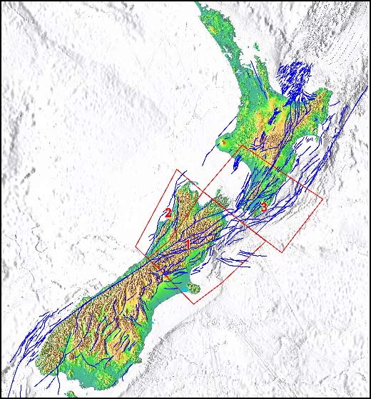
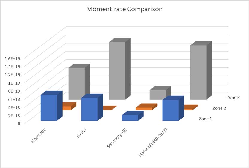
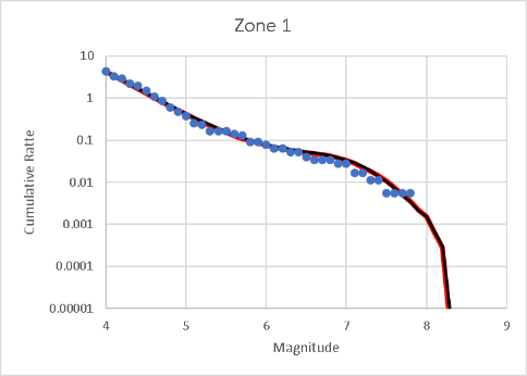
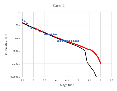
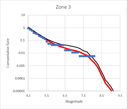
Figure 5 shows the impact of seismicity if the kinematic moment rate is used as a constraint. The seismicity model without the kinematic moment rate constraint is similar to the 2012 national seismicity hazard model for New Zealand (or the GNS2012 model, Stirling et al., 2012). For Zone 1, the seismicity model is almost identical with and without the kinematic model constraint. For Zone 2, however, the GNS 2012 model may have underestimated the rate for earthquakes with moment magnitudes larger than 7.2 (Mw> 7.2). For Zone 3, the GNS model may have significantly overestimated the rate of Mw> 7.0 earthquakes.
The application of kinematic modeling to time-dependency and tsunami modeling can be illustrated in the example of southwestern Japan. The subduction zone fault in the Nankai Trough has been ruptured in several great earthquakes since 1700. Block kinematic models were able to resolve detailed slip rate accumulation along the fault in the past few decades. Using the kinematic results along with the long historical earthquake record, we can obtain the current seismic slip accumulation (or deficit slip) along the fault (Figure 6). The accumulated slip along the fault can not only help calculate the time-dependent probability, but also the coseismic distribution of potential future large earthquakes, which is very important to detailed tsunamic modeling for megathrust earthquakes in the trough.
In developing an earthquake model for a region, AIR seismologists must estimate where potential future earthquakes are likely to occur, as well as how often they will occur and how big they will be. The strain rate field depicted in Figure 4 represents the distribution of seismic energy accumulation and is therefore indicative of where crustal earthquakes will occur in the future. But it also represents an energy "budget" to be spent by the occurrence of earthquakes. But will the budget be spent by frequent smaller events or by infrequent larger ones?
The historical record provides guidance on this question. If the historical record—which is dominated by the more frequent small-to-moderate earthquakes—effectively uses up the energy budget, then the historical record can be assumed to be representative of what will happen in the future. That is, the rate of occurrence of future earthquakes can reasonably be estimated based on the rate of occurrence in the historical catalog.
However, if there is an accumulation of energy that remains unspent by earthquakes in the historical record, a seismic "deficit" exists. Such a situation would indicate that, in that area, there is an increased potential for large infrequent earthquakes to take place. In this way, kinematic modeling and the energy accumulation rates it produces provide the guidance necessary to estimate the size and frequency of those large events whose return periods are close to or longer than the historical record.
Estimating the location and frequency of earthquakes that have long return periods is centrally important to seismic risk assessment. Yet, as outlined above, the historical and paleoseismic records are spotty at best and provide limited guidance. Kinematic modeling offers a physically based approach to understanding earthquake occurrence. As such, the shortcomings of a purely statistical approach can be effectively bypassed and the occasions when judgment has to be exercised are significantly reduced. Thus, kinematic modeling makes for a more robust model that reliably captures the risk from earthquakes—including those large events that have no historical precedence. The national seismic hazard model for Japan did not capture the risk from megathrust earthquakes and the Tohoku earthquake in the Japan Trench in 2010, one of the main reasons being that it was overly reliant on historical data, while largely having ignored results from kinematic modeling. For New Zealand, the Hikurangi subduction zone, which is the largest fault impacting the country, has not had any large magnitude earthquakes in the known history. While New Zealand residents have experienced many tsunami waves in the past 150 years, the most significant came from distant earthquakes such as offshore of Chile and Peru, not from local fault sources. The national seismic hazard model for New Zealand in 2002 did not consider any risk from earthquakes with magnitudes larger than 8.5 in the Hikurangi trench, due to the lack of a historical record of earthquakes larger than magnitude 8.0 in the trench. In 2012, the national seismic hazard model for New Zealand was updated to include scenarios as large as M9.0 based on the result of kinematic modeling and lessons seismologists learned from the Tohoku earthquake in Japan.
AIR anticipates the release of our updated New Zealand Earthquake Model in 2019, which considers the risk of megathrust earthquakes in the Hikurangi trench, based on kinematic modeling results for both the shake and tsunami models.