Modeling Fundamentals: FAQs about Average Annual Loss

Q: What is the relationship between AAL and loss cost?

A: AAL, which is a rough measure of the absolute “riskiness” of a set of exposures, is highly dependent on the underlying value of the portfolio. A high AAL, for example, could indicate that a portfolio contains high exposure value or that the exposure is at high risk of loss to the perils under examination, or both. The loss cost, on the other hand, is a measure of the relative risk of a set of exposures. It is calculated by normalizing the AAL per USD 100 of exposure.

Q: How is the shape of the EP curve reflected in the AAL?

A: As discussed briefly in "What Is AAL?," the shape of the EP curve is determined by the nature of the peril, the region, and the portfolio under analysis. Likewise, the contribution to the AAL from the different parts of the EP curve is affected by its shape. One general way to characterize this relationship is by measuring how much the distribution leans to one side or the other of the mean, or AAL. There are many ways to quantify this asymmetry, but for our purposes, we will use TVAR/AAL, where TVAR is the tail value at risk (the expected value beyond a given exceedance probability).

Low frequency/high severity perils like earthquake tend to be more asymmetrical, and the degree of asymmetry varies not only by peril, but also regionally within a peril. For example, the distribution of earthquake losses for the New Madrid Seismic Zone (NMSZ) exhibits much more lean than that for California (see Figure 1). This is because large NMSZ losses are far more infrequent than in California and are expected to occur only once every 500 to 1000 years, on average.

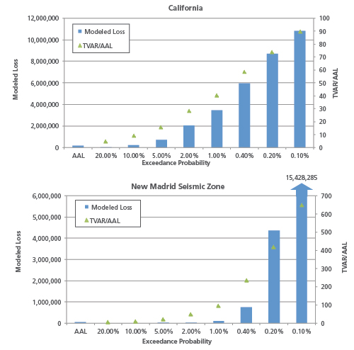
The shape of the EP curve also provides some insight into what is driving risk to the portfolio. In the above example, the shape of the NMSZ distribution indicates that the low frequency portion of the curve contributes more to the AAL than the high frequency portion. For California, losses beyond the 500-year return period account for approximately 15% of the AAL. For NMSZ, losses beyond the 500-year return period account for more than 80% of the AAL, indicating that relatively rare events are making up the bulk of the AAL.

Q: Does a larger standard deviation imply greater uncertainty?

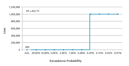
A: The standard deviation of the exceedance probability distribution is taken into consideration in many standard policy pricing equations. In its most basic sense, standard deviation is a measure of how much variation the portfolio-level EP curve exhibits from the mean of the distribution, in this case the AAL. As such, it is reflective of the nature of the peril and is not a pure measure of uncertainty in the loss calculation.

In a highly simplified (albeit unrealistic) example, suppose that a certain fault ruptures with the regularity of clockwork—always with the same magnitude and exactly every five hundred years. Because losses are zero in 499 out of 500 years, the standard deviation is high, but the uncertainty in the distribution and its AAL is zero (assuming, also, the same exposure at risk over time).

A way to normalize the standard deviation (SD) to compare different sets of analysis results is by calculating the coefficient of variation (CV), which is SD/AAL. In essence, a large SD may not be all that alarming if the AAL is also very large. However, a high CV—associated with low frequency/high severity phenomena—usually implies a higher degree of uncertainty. Knowledge about low frequency phenomena is inherently more limited.

Q: What is the impact of catalog size on AAL?

A: AIR typically generates a very large (50,000-year, 100,000-year, or even 1 million-year) set of simulated events and extracts a subset to produce the standard 10,000-year stochastic catalog included in the software. The AAL calculation methodology is the same regardless of catalog size; larger catalogs just mean that losses are averaged over a larger number of years. Because AAL represents a long-term average, it should not be expected to change significantly when calculated using a larger sample.

AIR's extraction methodology is such that the smaller optimized catalogs carefully preserve metrics from the larger sample, including frequency/intensity distributions. The Law of Large Numbers states that a large number of trials will exhibit convergence to a mean value; 10,000 trials are typically sufficient to establish this convergence and the mean is thus not expected to change markedly with more samples. Using a simpler everyday example, we would not expect that the average height of a population to change significantly based on a random sample of 50,000 individuals compared to one with 10,000 individuals.

Of course, larger event catalogs are able to capture more severe losses beyond the lowest exceedance probability point of the smaller catalog and offer more complete spatial coverage. The effect of these higher losses on the AAL is offset by their rarity. Furthermore, the larger catalog should not be regarded as entirely separate from the 10,000-year catalog. For example, the 10,000-year catalog is contained in its entirety in the 50,000-year catalog, so a significant portion of the 50,000-year average is already accounted for by the 10,000-year average.

Q: How is AAL validated?

A: A common mistake is to use the annual average loss from the available loss history to validate the modeled AAL. However, the modeled AAL is based on 10,000 or more years of simulated activity, and thus cannot be directly compared with the observed AAL based on historical data, which typically extends no more than a few decades. Indeed, the purpose of a model is to enable risk managers to look beyond the limited historical data for a better understanding of what is possible.

For example, according to data from the Insurance Council of Australia, bushfires in Australia have caused annual average losses of AUD 123 million over the years 1967-2011. Again, because the historical data is limited and has likely not captured more extreme events that are possible, this historical AAL should not be directly compared to the modeled AAL from AIR's 10,000-year historical catalog, which is roughly AUD 200 million.

To make a meaningful comparison, it is first necessary to isolate losses from an analogous range of exceedance probabilities from the stochastic catalog. One way to do this is to benchmark the highest historical loss in the data set against the modeled EP curve to determine the corresponding return period. Then, using modeled losses only up to this return period, the modeled AAL can be calculated and then compared to the historical AAL. The highest loss in this bushfire example corresponds to an exceedance probability of 2% (or a 50-year return period). Taking only modeled losses up to this exceedance probability, the modeled AAL is AUD 127 million, which compares very well with the historical AAL.