
Modeling Fundamentals: Evaluating Risk Measures
Jan 23, 2014
Editor's Note: Senior Vice President David Lalonde and Risk Consultant Alissa Legenza describe various risk measures that can be used when assessing capital and solvency requirements and pricing risk transfer opportunities.
Use of appropriate risk measures is crucial when assessing capital and solvency requirements and when pricing risk transfer opportunities, among many other business needs. When risk measures are not well understood, opportunities to optimize the allocation of risks are too often missed. It is therefore of fundamental importance that business decisions are based on the most robust measures of risk available. This article aims to promote awareness of the advantages and limitations associated with common risk measures. In addition, some lesser-known techniques for measuring financial risks are also examined.
Value at Risk
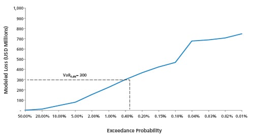
The financial industry began researching new methods for measuring exposure to downside risks in the late 1980s, following the infamous Black Monday stock market crash. It was then that value at risk (VaR) became popular as a risk measure. VaR is a single value from a loss distribution, often with an associated probability of exceedance.
The insurance industry later adopted the widespread use of VaR as a measure of catastrophe risk. During the early years of its use, VaR was often confused with probable maximum loss (PML); however, it is not the maximal or most probable extreme loss. Rather, VaRp indicates the minimum loss that is likely to be met or exceeded in a given year for a given level, p, of probability. In mathematical terms, if we define a random variable, X, as the annual loss, VaR is the loss, πp, that has a corresponding annual exceedance probability of p.
VaRp(X) = πp
P(X ≥ πp) = p
The use of a single value to represent an entire risk profile may be a tempting option for decision-makers—especially for regulators and rating agencies, which require intuitive measures that can be easily adopted when comparing risk profiles across many peer companies. However, VaR cannot tell the full story of a company's exposure to financial risks.
Figure 2 shows a plot of simulated hurricane losses for two companies (Company A from the previous exhibit and a peer Company B). Can you tell which company is riskier based on the VaR0.4% level alone? The answer, of course, is no. Comparing the two companies based on a single point value fails to demonstrate that each company varies in exposure to risks at different exceedance probabilities. For example, Company A's risk profile indicates that it may be at risk to larger and more frequent losses than Company B below the VaR0.4% level. On the other hand, Company B is riskier than Company A toward the tail of the risk profile, meaning that Company B may experience more significant losses than Company A, should a less likely but more extreme disaster occur. This information is not apparent based on the VaR0.4% level alone.
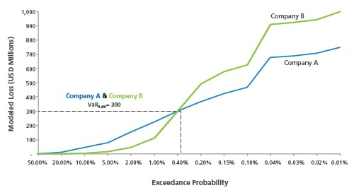
VaR can exhibit large variations after even minor adjustments to the underlying exposure data or to model assumptions. VaR also fails to capture the severity of extreme loss-causing events in the tail of the loss distribution, beyond the probability with which it is associated. This clearly becomes problematic for stakeholders who aim to hedge tail risks, especially for making catastrophe reinsurance purchasing decisions or for assessing capital-based requirements. Not surprisingly, VaR has become an outdated measure for catastrophe risks.
Tail Value at Risk
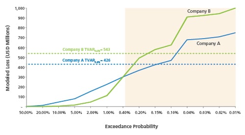
A risk measure commonly used in catastrophe risk management today is the tail value at risk (TVaR). TVaR measures the probability-weighted average, or expected value, of simulated event losses at or exceeding a specified VaR and is a more appropriate statistic for measuring catastrophe risk. TVaR is a conditional expectation that reveals how great financial losses could be, on average, given that a severity threshold has been exceeded. Mathematically, TVaR is defined as follows:
TVaRp(X) = E[X|X ≥ πp]
TVaR belongs to a family of risk measures that satisfies the properties of "coherence" (see sidebar), which are said to encourage the diversification of risks and reduce exposure to model uncertainty. In contrast, VaR fails the (subadditivity) test for coherence.
TVaR has become more widely accepted among stakeholders in the insurance industry. For rating agencies and other stakeholders who focus on tests for solvency during periods of extreme downside risks, TVaR can be an appropriate measure.
The drawback to TVaR is that it is not quite as intuitive as the VaR measure. And like VaR, TVaR is also sensitive to changes in underlying model assumptions—in particular, those that affect the tail of the loss distribution. In addition, while TVaR is an improvement over the VaR measure, it may not be necessary to take into account the few events that make up the remote tail of the loss distribution for reinsurance pricing decisions. Most insurers do not find it economically feasible to protect against such events and as a result do not purchase catastrophe reinsurance for these extreme disaster scenarios.
Window Value at Risk
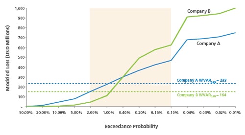
Another risk measure to consider is called window value at risk (WVaR). This measure takes the probability-weighted average of a distribution of losses within a range of practical bounds, or percentiles, and can be mathematically described by the following formula:
WVaRp,q(X) = E[X|πp≤ X ≤ πq]
WVaR is less sensitive to changes in the tail resulting from updates to the underlying model or exposure data and generally exhibits less volatility than other risk measures as a result. Most importantly, risk managers can apply practical bounds that represent the appropriate range of losses to support their risk management needs. This eliminates the need to reflect extreme losses at the tail of the distribution in decision-making processes.
Tail Value at Risk Calculation in AIR's Touchstone® Software Platform
TVaR represents the probability-weighted average tail loss for a particular contract/portfolio. The TVaR at a specified exceedance probability is obtained by finding the average of all event losses at that exceedance probability and lower. This can be done on both an occurrence and aggregate loss distribution. Given an AIR catalog containing N event years, the probability of each event loss, Li, is 1⁄N. TVaR can then be formulated as follows:
For a catalog size of 50,000 event years, for example, the TVaR0.99 (X) can be expressed as:

Censored Tail Value at Risk
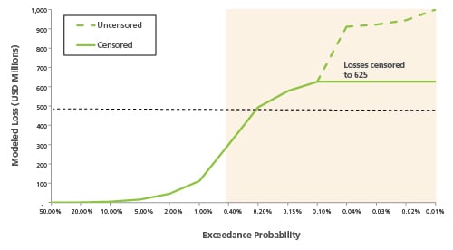
While window value at risk does improve over tail value at risk by ignoring the extreme loss behavior that exists in the tail of the distribution, is this the ideal approach? Perhaps the ultimate technique for measuring exposure to catastrophic risk could be accomplished by restricting, rather than ignoring, the tail domain of the loss distribution. Simulated event losses that fall outside of the range of what might be considered economically feasible to protect against could be censored, or capped, prior to applying the same conditional expectation methods used to calculate the tail value at risk.
This special case is a censored tail value at risk, or CenTVaR, and can be derived by the following formula:
CenTVaRp,πq(X) = E[X|πp ≤ X ≤ πq] + Pr(X > πq) × πq
πq = censored event loss value
The final case study, depicted in Figure 5, examines the censored tail value at risk measure for Company B.
Risk Measure Comparison
This article has presented simplified case studies for measuring exposure to catastrophe risk across two peer insurance companies. What final conclusions can be illustrated for these peers with regard to exposure to U.S. hurricane risk? Table 1 provides the risk measurements previously discussed for each company. The TVaR0.4% and CenTVaR0.4%, $625M measures indicate that Company B is exposed to more risk than A at the higher return periods. However, Company A is exposed to more risk than B at the lower return periods.
| Peer Company | VaR0.4% | TVaR0.4% | WVaR2.0%, 0.1% | CenTVaR0.4%, $625M |
| A | 300 | 426 | 233 | 416 |
| B | 300 | 543 | 164 | 488 |
Determining which company is riskier overall depends largely on which business application is used and what the interests of the decision-maker are. For example, business managers and investors are typically focused on measuring prospects for earnings (or deficits) reflected in the lower return periods of the loss distribution. Conversely, rating agencies and regulators are concerned with a company's ability to remain solvent and, therefore, look to measure risks in the higher return periods of the loss distribution.
Conclusion
Choosing an appropriate risk measure is critical for stakeholders in the insurance industry who must demonstrate ownership of their risk. Proper evaluation of risk measures can help risk managers facilitate the analysis of risk across regions, perils, and multi-year horizons. By understanding the strengths and weaknesses of different risk measures, setting levels to reflect risk appetite, and considering how they combine with other constraints over a planning horizon, stakeholders will be well prepared to manage the next extreme disaster event.
1 Artzner, Philippe; Delbaen, Freddy; Eber, Jean-Marc; Heath, David (1998). "Coherent Measures of Risk"(pdf). Pp. 6- 7