
In the cat modeling world, we often model variables (such as losses or hurricane central pressure) based on their distributions in the historical data. We usually find a distribution whose properties are well understood, fit it to the historical data, and proceed. Sometimes sampling from non-standard distributions is needed because the well-understood distributions do not fit the data well; in other cases, we need to find an association between two distributions.
In the latter cases, the rejection sampling technique can be used to generate samples with complicated distribution via sampling from some simple distributions, or to obtain samples that fit the characteristics of one distribution from another distribution.
Rejection sampling is a Monte Carlo sampling method such that the samples are drawn from a proposal distribution and, after the rejection process, the kept samples are distributed according to the so-called target distribution. The requirements for the proposal distribution are straightforward: It should be easy to sample from and must cover the entire range of the target distribution. Another implicit requirement is that both target and proposal distributions be capable of being evaluated for different values in the range.
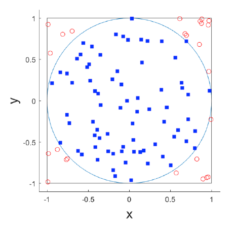
Figure 1 shows a simple use case of rejection sampling: sample uniformly distributed points inside a unit circle centered at ( 0,0 ). In other words, everywhere inside the circle has an equally likely chance to be sampled. A simple implementation based on the rejection sampling principle would be:
1. Draw a pair (x, y) from a uniform distribution with range [-1,1]. (Clearly each pair is within a square with width 2.)
2. Accept the pair if x2 + y2 <1 (see the blue squares in Figure 1), reject the pair otherwise (see the red open circles in Figure 1).
In the end, we wind up with samples (i.e., x-y pairs) that are distributed uniformly inside the circle. In this case, our target is samples distributed uniformly inside a circle, and our proposal is samples distributed uniformly inside a square bounding the circle.
Now imagine that the points inside the circle do not distribute uniformly, i.e., there are more points in some places and fewer in others (see the blue curve in Figure 2). Can we still use the rejection sampling technique to obtain points with such a distribution? The answer is yes.
Figure 2 illustrates the steps of rejection sampling for a much more general case. In the figure, the blue curve is the target distribution (p(x)) we want to achieve, and the dashed rectangle is a proposal distribution we use (q(x))—a uniform distribution in this example. The procedure is as follows:
- Select a proposal distribution q(x) that covers the x range.
- Find a constant C so that Cq(x) ≥ p(x) for every x.
- Draw a sample (say x1) from distribution q.
- Calculate p(x1) and Cq(x1).
- Draw a sample (say u1) from a uniform distribution with range [0, Cq(x1)].
- Keep (i.e., accept) x1 if u1 ≤ p(x1). Throw it away (i.e., reject) otherwise.
- Repeat Steps 2-6 until the sample size (i.e., how many x we want) is reached.
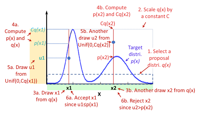
Again, in the end, all x accepted would look like they are drawn from distribution p(x). A variant of Steps 3-6 is to draw a random number u from a unit uniform distribution, compare u with ratio p(x1)/Cq(x1), and reject x if u > p(x)/Cq(x).
In addition to the requirement of the sample space coverage, a proposal distribution should also be chosen to optimize sampling efficiency. If the proposal distribution is vastly different from the target distribution, many samples will be rejected before a sample is accepted, thus the sampling efficiency would be low and it would take a long time to reach the sample size desired. If there is a choice, we would use a proposal distribution that produces a high acceptance rate, which is the ratio of the number of samples accepted over the total number of samples drawn.
The rejection sampling technique differs from the Markov Chain Monte Carlo sampling method in that it does not have a so-called “burn period,” within which samples need to be discarded before they are considered as relevant. In other words, all accepted samples generated from the rejection sampling procedure are good to use.
An Example
A useful application of the rejection sampling technique is to reconstruct the longer historical record from a recent (shorter) record. One difficulty in the hurricane simulation business is that while data for the number of hurricanes and landfalls in the U.S. are considered reliable since 1900 (a relatively long record), atmospheric environment data—such as the Climate Forecast System Reanalysis data from the National Centers for Environmental Information, National Oceanic and Atmospheric Administration—go back only about 30 years, a much shorter record. Therefore, simulations based on the recent environmental data may not represent the longer historical record. One approach would be to resample the simulated hurricanes generated from the shorter record via the rejection sampling technique so that they emulate the 1900–2017 period.
We use the Multivariate El Niňo Southern Oscillation Index (MEI) and the extended MEI for this exercise. (For this purpose, the association between MEI and hurricanes that we need to know is that more hurricanes are expected during El Niňo years and fewer in La Niňa years.) The goal is to resample the El Niňo-Southern Oscillation (ENSO) signals from the record of 1982–2017 so that they represent those from the 1900–2017 period.
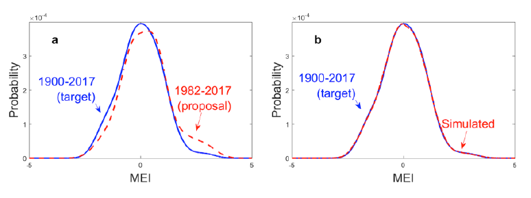
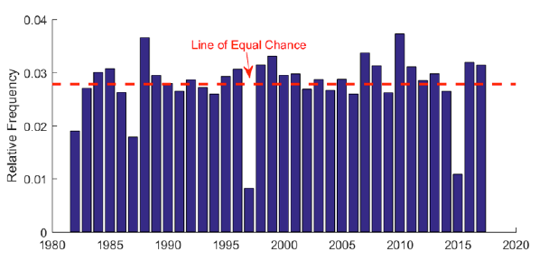
Figure 3 shows the target and proposal distributions and the end results. Chart a indicates that more El Niňo years occurred in recent years than in the longer record, thus, we need to correct for the overrepresentation of the El Niňo signals. After sampling each year of the 1982–2017 period for different times (via rejection sampling), the end results, with the bias of large ENSO signals largely corrected, resemble a distribution of the 1900–2017 record. Tracing back the number of times each year's MEI value was sampled, we can obtain information about the number of times each year that needs to appear in the final assembly for it to look like the 1900–2017 record (Figure 4). Years with strong ENSO signals were clearly undersampled (especially 1982, 1987, 1997, and 2015) while years with negative MEI values were oversampled. This exercise demonstrates that to some extent we can compensate for the lack of historical record by using the rejection sampling technique.
To conclude, rejection sampling is a simple but useful sampling technique that has many applications in the field of cat modeling and hazard simulation. It can be extended to multi-dimensional problems, which I'll discuss in my next blog.