Editor’s note: This blog was also published on the website of the loss modeling framework OASIS

The Oxford English Dictionary defines “counterintuitive” as that which is contrary to intuition or common-sense expectation. When I hear the word “intuition,” I think of something innate and untaught yet often improved by experience. Where we can get into trouble with our intuition is when we rely on it for things outside our experience. In this article I demonstrate some of intuition’s pitfalls and argue that being aware of these pitfalls is vital to prevent falling victim to them.
Typical life experience doesn’t really prepare you well for developing an intuition for the metrics of cat modeling. For example, it does not generally lend itself to developing an intuition for the consequences of an M7.5 earthquake in Downtown Los Angeles. Intuiting the financial fallout from a hurricane, on the other hand, may be somewhat less challenging because such storms are more frequent. In either case, the sophisticated insurance practitioner will likely have the sense to doubt her intuition and rely instead on analytics. Indeed, I’ve previously argued that an inability to relate a probability distribution to real world experience, as can be done so readily with hurricanes for example, can have the insurance practitioner at a loss as to where to expect results involving probability distributions.
For example, if a ground up loss is X and there is a deductible Y, what should the gross to ground up ratio be? Gross losses are greater than (X - Y) when Y is applied to a probability distribution with mean X. Even knowing that, should the gross be 10% larger than X - Y or more? Of course, this depends on many factors such as the specifics of the probability distribution of X, but the point is that predicting the result intuitively can be difficult. Experience can provide some guidance, but when going outside the bounds of what you’ve experienced—for example a different probability distribution or peril—prediction is fraught with uncertainty.
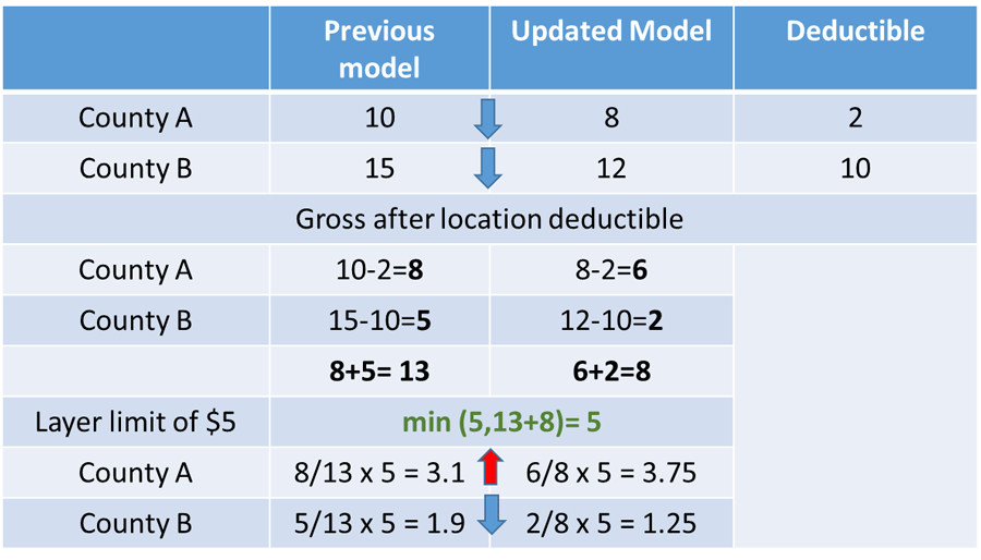
Financial results are also capable of not obeying laws we think are intuitive. For example, we would assume that, for any given wind speed, if the ground up loss is larger in one version of the model than in another, then the gross loss would also be larger. But that's not necessarily the case. See Figure 1 assuming two locations, each having a loss in County A and County B, respectively.

Then there are more gnawing examples of issues with intuition, issues stemming from perhaps unconscious but deep biases. Kahneman, in his book Thinking Fast and Slow, calls this thinking fast, and one of the biases I see us making is the availability heuristic. In this case the easier it is to recall the consequences of something, the more salient those consequences are perceived to be.
Take the 2011 Tohoku earthquake, for example; if asked what proportion of the overall loss was due to tsunami, many people would say more than half (the answer, from claims, is about 20%). Perhaps participants are recalling images of the waves rolling inland, taking with them houses, automobiles and, tragically, people. But lower severity damage for most events is much more widespread. In the case of Tohoku, lots of locations with lower severity shake damage over a wide coastal and inland area accounted for more loss than the relatively narrow coastal strip of complete devastation.
I see a similar line of thinking in audiences I ask to estimate the return period of Hurricane Katrina. Many respondents say 50 to 100 years, possibly recalling the scale of the devastation. But it’s actually closer to 25 years when you plot the loss from a recurrence of Katrina today on a U.S. hurricane occurrence exceedance probability (EP) curve.
Perhaps intuition isn’t so great at putting losses on EP curves correctly. But is that what your intuition is doing? I’d imagine the audience respondents in my example probably aren’t putting a loss on an EP curve (unless they have stellar memories), but rather their responses are based on the expected frequency of loss in X number of years. Realistically, though, they’d need pen and paper and some losses to answer correctly, which leads me to think we shouldn’t answer questions on return periods using our intuition but only after doing some analysis.
Although we discuss return periods above, this term can sometimes be prone to misinterpretation. A 100-year return period loss does not mean a loss that recurs every 100 years, but rather a loss that has a 1% annual probability of being exceeded. Thinking in these annual terms, however, is also prone to its own biases whereby individuals’ risk perceptions can change by framing the risk over a longer period of time. According to Botzen, Kunreuther et al, framing the chances of a flood as being greater than 1 in 5 over 25 years rather than 1 in 100 in any given year could impact risk perception and make property owners more likely to take flood risk seriously.
Recency bias can also affect our intuition. After the 2004 and 2005 Atlantic hurricane seasons there was some market consensus for a "near-term view of hurricane risk" due to the assumption that the risk landscape had fundamentally changed. Contrast this with the 10-year hurricane drought that followed.
One example we sometimes see is the impact on average annual loss (AAL) of adjustments to an EP curve. Seasoned cat modelers know that AAL impacts require thinking about both frequency and severity. So AAL with and without tsunami may only be 0-2% different, depending on the region. This can be counterintuitive to some, but recall the rarity of damaging tsunamis—AAL divides the entire catalog’s losses by the number of years in the catalog, and many years contain no tsunami loss.
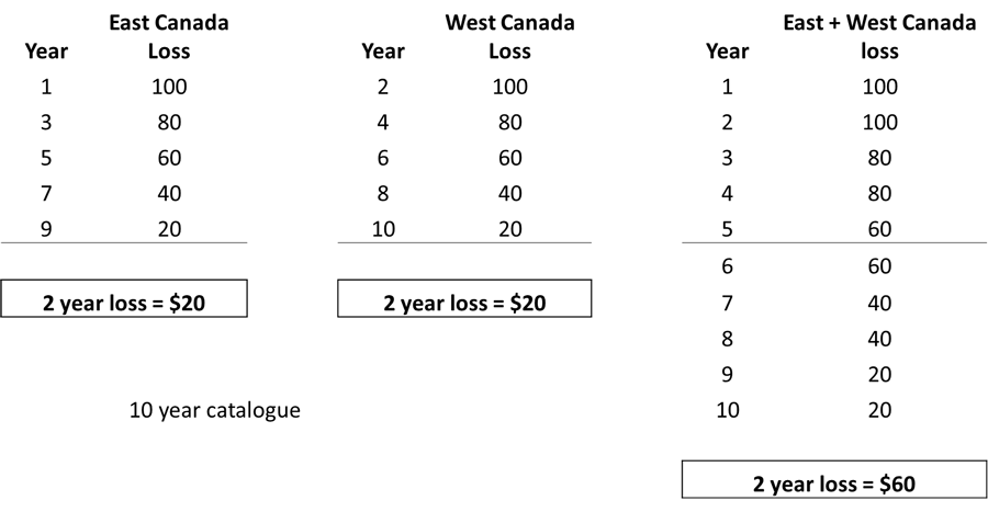
Finally, what of that wily metric we use so often, EP loss? When you add portfolios A and B together, their risk metrics should yield to some diversification. That is, Risk Metric (A+B)<=Risk Metric (A) + Risk Metric (B). But alas exceedance probabilities (and return periods) don’t show that behavior (TVaR, tail value at risk, does). In some instances, you may (counterintuitively) find that adding two portfolios increases the overall risk, a circumstance called super additivity where RP(A+B)>RP(A)+RP(B). See Figure 2 for an example where this occurs; some would expect the combined RP loss for two portfolios in the same region A+B to be less than the value for the RP losses after adding A and B separately.

As I’ve shown, intuition isn’t always perfect, so learning its pitfalls is important to prevent falling into its traps. Do let us know if you have any counterintuitive examples you’d like to share!
Read about the calculation of average annual loss (AAL) in “Modeling Fundamentals: What Is AAL?”


