Another U.S. hurricane season is just starting up, so it’s a good time to take a look at how demand surge could impact losses this year. Over the past 15 years, there have been a few extremely destructive seasons followed by many years that left little or no impact. This time period also saw a housing boom, followed by a housing market collapse that left many regions struggling to recover for several years, particularly Florida.
The global recession in 2009 had an impact across the U.S. construction market that led to a lot of excess capacity, followed by a decline in construction employment. In recent years, however, there have been pockets of recovery in the construction industry. The U.S. is made up of hundreds of local construction markets, each reflecting local needs and setting its own baseline of activity that can determine the demand surge response after an extreme event.
Transposing Charley
The easiest way to understand how the coming season might look is to revisit a prior event and place it in the context of the current economic environment. Hurricane Charley, which made landfall in Florida in 2004, would be a good choice. By itself, it wasn’t all that impressive, but it struck during a time of unprecedented construction activity and was the first of several storms to impact the state during the height of the construction boom over two hurricane seasons. Employment was growing by double digits annually by 2002 in many local construction markets in Florida.
Figure 1 charts the quarterly levels of construction employment in Florida prior to the start of the hurricane season in 2004 through 2016, and the quarterly levels of construction permits. Both time series have been seasonally adjusted using a centered moving average and are represented in thousands of units. To give perspective, the 2004 hurricane season is indicated by the vertical line. What sticks out is that the changes in employment follow the changes in construction permits. Before 2005, the employment level follows the track closely, with the ratio of permits to employees close to 1. After 2005, permit levels fall much more dramatically than employment, with the biggest gap in 2009. This is where we see excess capacity, even though employment is falling. Through 2016, the gap continues to narrow but never returns to the tight labor markets before 2005.
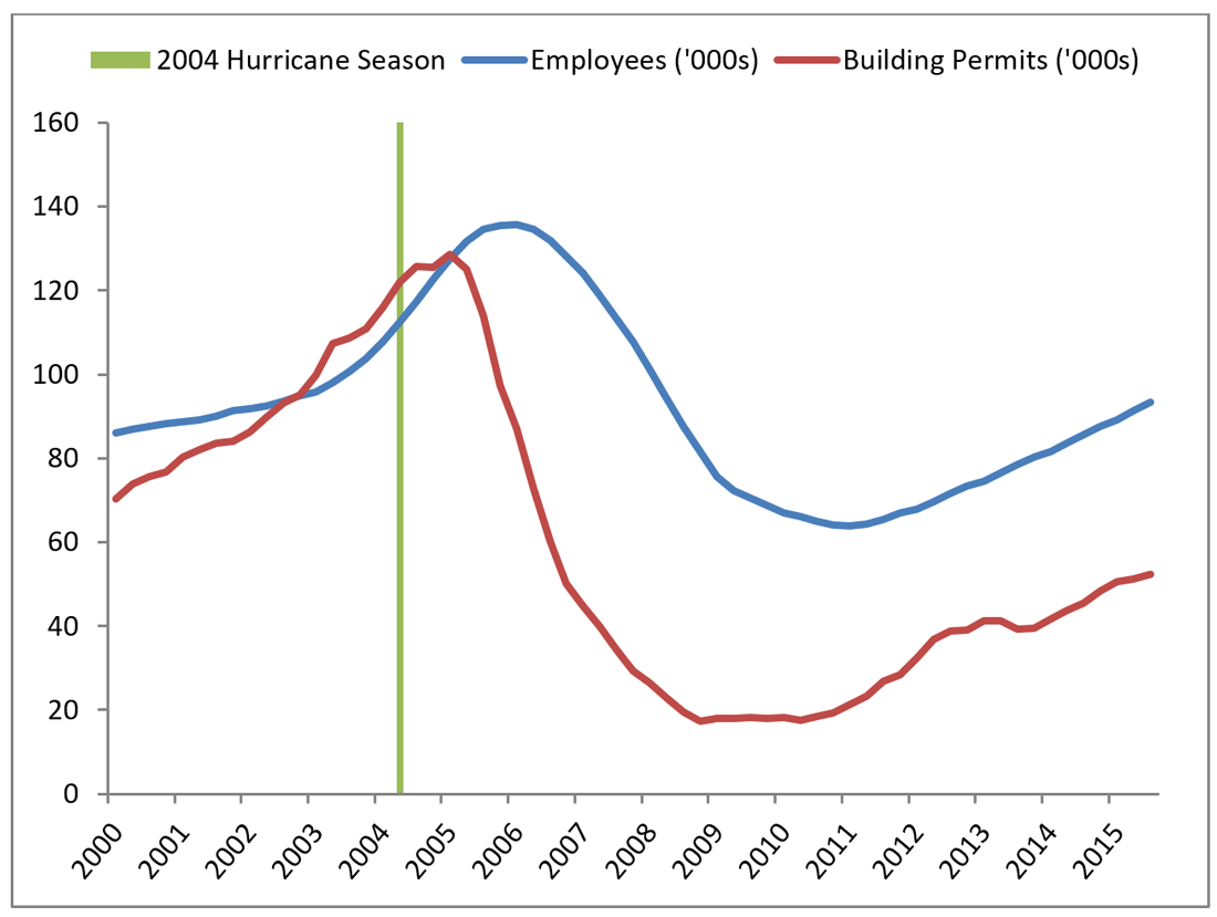
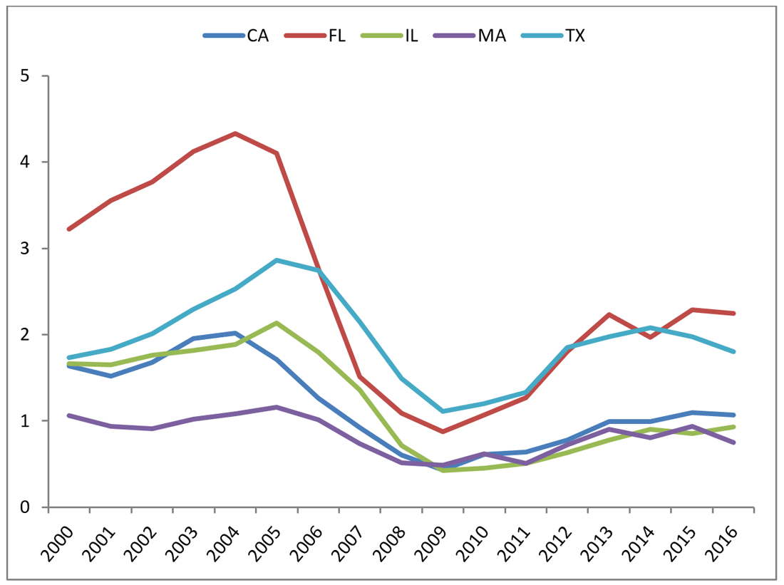
Figure 2 charts the number of annual construction permits per construction employee in five U.S. states from 2000 through 2016. This metric is interesting because it compares future demand (current permits) for construction with the employment levels at the time. What immediately jumps out is the metric for Massachusetts (MA). Throughout the housing boom, recession, and recovery, the ratio remains at a stable value consistent with normal construction trends. California (CA) and Illinois (IL) are a little more active during the housing boom years, but after the recession follow a trend similar to that of Massachusetts. During the housing boom era (2000 to 2005) there was a huge demand for future housing, but the highest metrics in the U.S. were seen in the southeastern part of the country—represented here by Florida (FL) and Texas (TX). While Texas was a hot market, Florida was sizzling and had the farthest to fall after the recession hit. Florida and Texas have since followed a similar pattern of being more active than other parts of the country, but nowhere near as active as during the boom.
Normal Cost Inflation
The current state of the local construction market only tells part of the story. What this scenario is missing is straightforward, but far from simple—normal cost inflation. At AIR Envision 2017 I talked about demand surge model development and how it is important to remove normal cost inflation to measure how much of local cost increases can be attributed to the intensity of damage from an event. When looking at actual events that have already happened, it is fairly easy to identify cost inflation to subtract . But to get the complete picture of the impact on losses after an event today, it is important to understand the range of possible cost inflation and account for what might happen in the future by adding it back in.
There are two sources of cost inflation to look at separately: labor and materials. After an extreme event, the price of labor in the area immediately affected can increase beyond the normal labor cost inflation for years as claims are settled and the demand and supply of labor returns to a long-run equilibrium. I talked about this in my last blog post. The local materials market operates on a very different timeline. After accounting for normal materials cost inflation, the local materials price increases only last for a short time—one to two quarters.
Looking Ahead
The big unknown is how to account for future cost inflation for labor and materials in the broader economy. It is straightforward to look back at prior seasons and identify normal cost trends, but making predictions about future cost directions can be challenging. Three reasonable assumptions come to mind:
- Continue with the most recent inflation trend. Inflation is a time series, and current state is a good predictor for the near future. The problem with this assumption is that demand surge is associated with longer claims settlement and rebuilding, usually two years.
- Take the long-term average. If this is higher than current inflation, it would be a more conservative view and less risky. If, on the other hand the current state is higher, it would be a better choice in this case.
- Take the worst case scenario and assume the highest inflation based on experience. This is the most conservative and least risky of the three.
To view the impact of Hurricane Charley today, the labor cost inflation factor and materials cost inflation will have to be combined. If we assume that the total cost of construction is made up of equal parts labor and materials, a straight average will give the right results. For this example, weighted inflation values run from about 2% for the recent trend to almost 10% for the worst case scenario. Putting it altogether with the current state of local labor markets affected by the event, the expectation for the coming hurricane season can be seen in Figures 3 and 4. The left-hand map of Figure 3 compares the original event using market conditions and cost inflation from 2004, with the right-hand map showing the most recent market conditions and cost inflation experience. The main driver of difference between the two is the weighted cost of inflation; historically it was about 6% compared to 2% over the past two years.
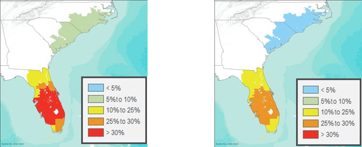
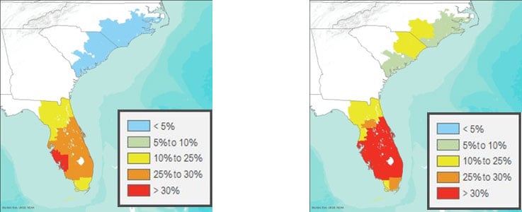
Figure 4 compares the current market conditions by using long-term cost inflation (left-hand map) and the worst case cost inflation (right-hand map). Using the long-term average results in a lower overall demand surge effect compared to 2004. For the worst case scenario, the demand surge map looks a little more intense than in 2004.
Demand surge is only one component of the loss inflation that can happen after an extreme event and because it can involve shortages of construction materials and labor, it is unavoidable. It transcends insurance losses because it affects all properties in the destructive path of a hurricane, insured or not. Other forms of loss inflation are more directly related to insurance and claims management, such as government intervention or a shortage of claims adjusters, and can vary from one insurer to another. It is also possible that a shortage of specialized construction labor that only affects a specific line of business can have an outsized effect on an insurer. Whatever the source of loss inflation, each component should be handled individually to get a better understanding of its impact on portfolio losses.