Optimizing Your Cat Bond Portfolio with a New LP Framework

Formulation for Mapping TVaR Topographically

Let f(x,y) be the loss associated with decision vector x and random vector y. The probability of loss not exceeding a threshold, α, can be denoted as:

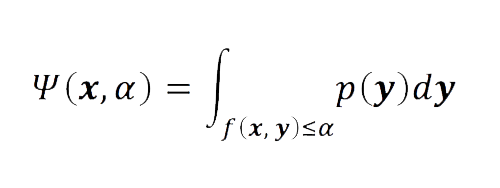
where p(y) is the underlying probability distribution of y, and Ψ(x,α) is the cumulative distribution function for the loss associated with x. Then VaR and TVaR for a point β ∈(0,1) can be defined as α _β and ∅ _β, respectively, where:

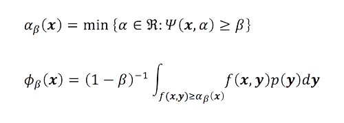
It can be shown that VaR and TVaR can be characterized by function F _β (x, α) and F _β (x,α):

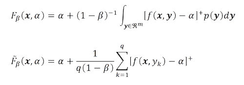
The function F _β (x,α) is convex and piecewise linear with respect to α, however it is not differentiable with respect to α. (This formulation is also known as the matrix notation. )

Implementation

Function F ̃_β (x,α) can easily be utilized in an LP problem formulation and, therefore, minimized. Standard linear programming problems can be structured as follows:

Min cx subject to
Ax ≤ br xi ≥ 0

Where
c = objective value coefficient vector
A = constraint coefficient matrix
b = right-hand-side value vector
x = vector of decision variables
i = index for the i^th decision variable

Structuring the portfolio optimization problem as an LP problem not only leads to improved computational efficiency but also enables pinpointing the exact optimal solution(s).

Constructing a full, working application of the LP framework to address portfolio optimization problems in the cat bond space requires several other components. To obtain simulated annual loss scenarios to evaluate the risk metrics TVaR and average annual loss (AAL), we can leverage the catastrophe bond database in AIR's CATRADER® system. Also, by running portfolio analyses by contract and zone in CATRADER, the information stored in CATRADER's loss database allows the LP portfolio optimization framework to place constraints related to peril, geography, and contract in A, the constraint coefficient matrix.

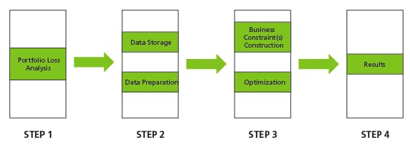
The portfolio optimization framework discussed in this article adheres to the workflow illustrated in Figure 1, a robust, flexible framework specifically tailored for the insurance industry. The framework is built to address various challenges, such as minimizing the portfolio risk without settling for a lower return or maximizing portfolio return without loading the portfolio with unnecessary risk.

Cat Bond Case Study

Addressing the portfolio optimization problem in the cat bond space effectively illustrates the practical application of the LP portfolio optimization framework for a couple of reasons:

• The cat bond space includes approximately 140 transactions. From an optimization standpoint, this means 140 relevant contract-level decision variables to consider across the entire market. This example is easily extendable to either additional cat bonds or a large portfolio of reinsurance contracts.
• AIR's catastrophe bond database (CBDB) contains thorough information—such as detailed risk analysis and issuance yields—on all the property deals in the market (that is, it currently excludes bonds covering life, mortality, medical claims, and private placements).

Our portfolio optimization case study, which will validate the capabilities of the LP portfolio optimization framework, solves for the following objective function: For a portfolio constructed at a given principal amount, what percentage of the portfolio should be allocated to each transaction in the market to minimize overall portfolio TVaR while retaining 7% expected return on principal invested? (The data for this case study consists of all transaction data contained in CBDB.) The challenge—minimizing TVaR while satisfying the 7% constraint—can be described as Portfolio_{(Expected Return)}≥7%.

Figure 2 illustrates the efficient frontier built around the 7% expected return threshold:

X-axis = portfolio/individual security TVaR as a percentage of the principal
Y-axis = percent expected return
red square on the curve = minimum portfolio TVaR at 7% expected return threshold
green triangles = individual securities (bonds) in the CBDB
blue square = hypothetical market portfolio

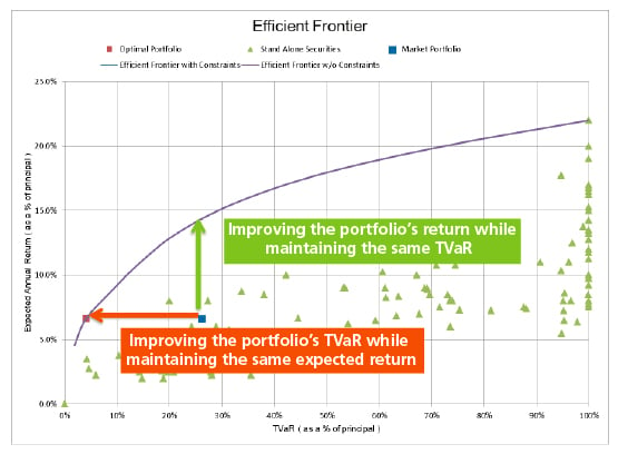
The curve in Figure 2 was built by varying the threshold for the expected return from approximately 3.5% (percent expected return of the lowest-yielding bond) to approximately 22% (percent expected return of the highest-yielding bond) and rerunning the optimization analysis multiple times. The blue square represents the hypothetical market portfolio constructed by investing 100% in each of the transactions that exist in our universe of cat bonds. Any cat bond portfolio that lies below the efficient frontier, including our hypothetical one, is clearly suboptimal; that is, for a given risk level the expected return could be vastly increased or, alternatively, for a given expected return the risk load could be dramatically reduced.

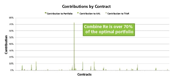
An interesting wrinkle emerges when we look at how the portfolio weights are distributed across all the bonds in the market. As shown in Figure 3—which indicates what portion of the portfolio should be assigned to each bond—the results of our optimization exercise (as represented by the red square in Figure 2) recommends that over 70% of the portfolio should be invested in Combine Re. This makes sense from a mathematical point of view because Combine Re offers a high expected return for a relatively lower risk load. However, from a business perspective, this is not a desirable outcome because it means putting all your eggs in the one basket, as the saying goes. Also, the market might not allow investing that large a percentage in a single bond.

The kind of unwanted concentration illustrated in Figure 3 can be easily avoided, however, if other constraints are introduced into the framework. For example, for the same problem if portfolio weights are constrained to no more than 10% (x_i≤0.1), the efficient frontier shown in Figure 4 is obtained.

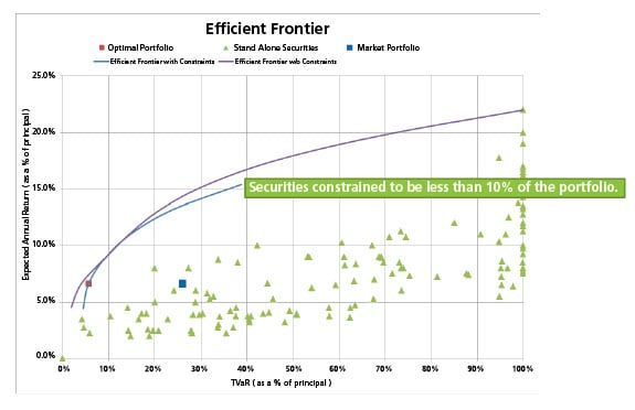
Figure 4 is identical to Figure 2 with the exception of the blue constrained efficient frontier curve. The constrained efficient frontier curve does not stretch as far out as the unconstrained curve because with the portfolio weights constrained to be less than 10%, achieving an expected portfolio return above roughly 15% becomes impossible. As Figure 4 suggests, the impact of the constraint can be dramatic.

This LP portfolio optimization framework also enables the construction of peril-related and geographical constraints—avoidance of over—concentration in transactions covering Florida hurricane losses, for example—that facilitate in-depth and realistic optimization analyses. Importantly, the framework can account for business challenges specific to the insurance industry, resulting in educated portfolio decisions.

Stress Testing

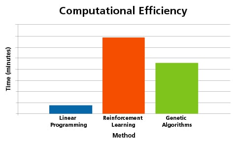
The LP framework described here can be used to solve a wide variety of other optimization problems, including insurance portfolio optimization. To test the computational efficiency of the LP portfolio optimization framework, we used books of 500-5,000 insurance policies. A series of optimization analyses was performed to validate the computational efficiency of the LP portfolio optimization framework. Using hypothetical portfolios, we observed the performance of the portfolio optimization framework and how computation time scales. For a portfolio of 500 policies, the LP portfolio optimization framework's performance was significantly better than other well-known algorithms used to address the same problem, as illustrated in Figure 5.

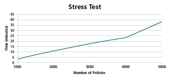
When dealing with smaller portfolios, the difference might not appear as significant from a practical point of view. However, when dealing with larger portfolios, the computational efficiency of the LP portfolio optimization framework scales linearly (as shown in Figure 6), while heuristic approaches scale exponentially.

Conclusion

The linear programming portfolio optimization framework maps a clear path of inputs to optimal portfolio decisions. Built around an LP formulation specific to the industry, the portfolio optimization framework offers the ability to yield exact optimal solution(s) very quickly. Importantly, the scope of the framework is not limited to cat bond portfolio optimization but can be extended to optimization problems in other market segments in the insurance industry, including primary insurance and reinsurance.

The second article in this two-part series will take an in-depth look at how we tailored the formulation to integrate with our modeled loss results and will discuss the reasonableness of the results.

For further information on AIR's linear programming approach to catastrophe bond portfolio optimization, please contact us at ILSsupport@AIR-WORLDWIDE.COM.