Optimizing Earthquake Catalogs for Better Model Performance

The Impact of Sampling Variability on Model Results: A Simple Example

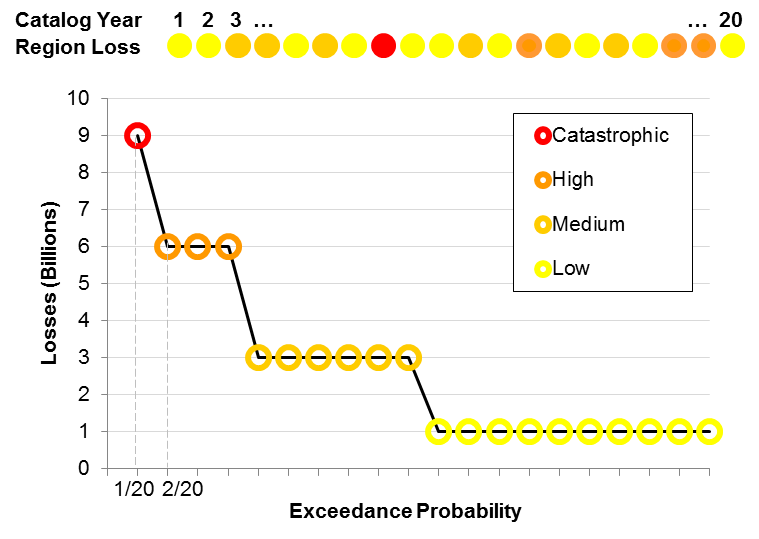
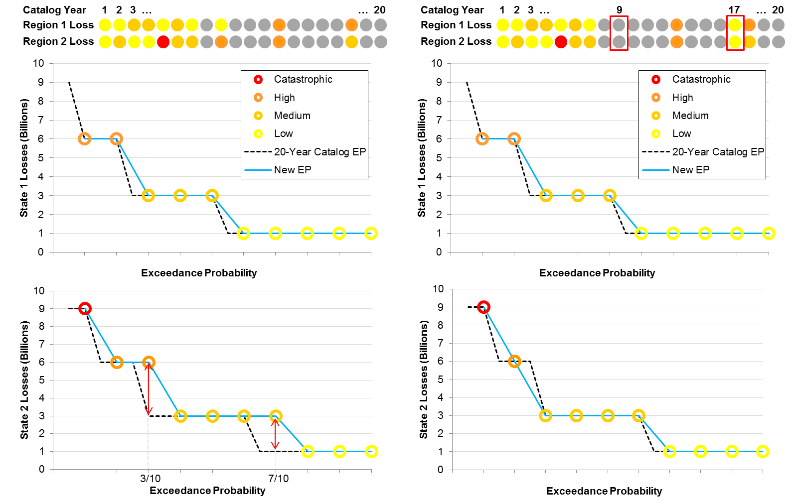
Suppose that we construct a stochastic catalog of only twenty years of potential catastrophe activity for a hypothetical model. Suppose also that the loss experience from these twenty years of activity in a given region can be categorized as low (1 billion) in 10 out of the 20 years, moderate (3 billion) in six of the years, high (6 billion) in three years, and catastrophic (9 billion) in one exceptional year.

Given this 20-year catalog, the loss exceedance probability (EP) curve is constructed by first ranking the losses from largest to smallest. The largest loss (9 billion) is equaled or exceeded only once in 20 years, so it is assigned the highest loss point in the EP curve (1/20) on the far left in Figure 1. Next are the three years of high loss, which create a plateau at the loss level of 6 billion, equaled or exceeded with a probability of 4/20. The rest of the curve is constructed in the same manner.

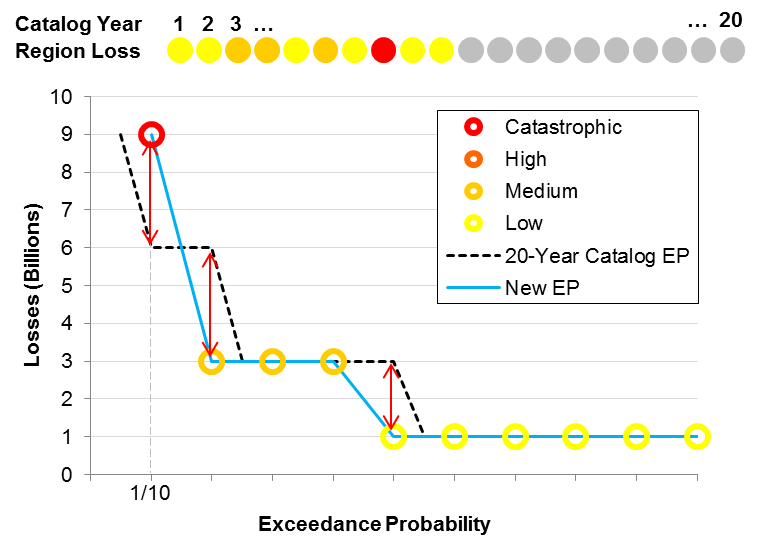
Let's assume that we need to speed up the computation process by extracting a smaller catalog of 10 years from the full 20-year catalog, while reproducing the EP curve shown in Figure 1 as faithfully as possible. The simplest extraction method is to randomly choose the first 10 years of simulated activity from the 20-year sample. Now, the probability assigned to each sample year is 1/10 because the catalog contains only 10 years of simulated activity. Accordingly, the exceedance probabilities of the highest and the second highest loss are 1/10 and 2/10, respectively. Figure 2 shows the result of this extraction and the corresponding EP curve.

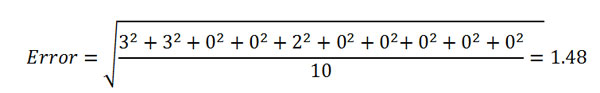
To determine whether this extraction has been successful, we need to quantify the overall difference between these two EP curves. One method is to measure the difference between the loss estimates at different exceedance levels, say 1/10, 2/10, …, and 10/10. At the 1/10 exceedance probability the difference in loss estimates is 9 − 6 = 3; at 2/10 the difference is 6 − 3 = 3; at 3/10 and 4/10, the difference is zero; and so forth. The total error, defined as the root mean square error, is

Is this the best we can do? Because this example is very simple, it is easy to conceive an alternative extraction that would yield much better results. Consider extracting sample years 13 and 18 from the 20-year catalog instead of samples 8 and 10. The result, shown in Figure 3, reproduces the EP curve from the 20-year catalog with a much higher accuracy according to our error metric. As a matter of fact, the error in this case, measured at the same probability levels considered above, is zero, meaning that the quality of this extraction is superior to just randomly picking the first 10 years.

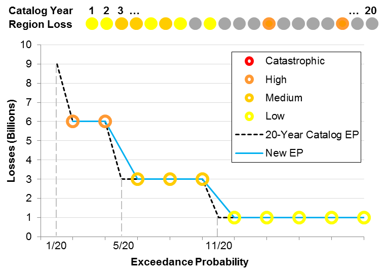
Note that there are some points from the 20-year EP curve that cannot be matched by this extraction, for example at 5/20 and 11/20. Similarly, the highest loss in the original catalog, at 1/20, is not captured in the optimized sample. While the EP curve is preserved more accurately than that of the random extraction, we lose sight of this potentially catastrophic year. Obviously, failing to represent an event with a 1/20 exceedance probability would be a problem in the real world, but AIR's catalogs are many orders of magnitude larger than that in this illustrative example. While losing the most extreme events is a numerically insurmountable challenge inherent to even the most sophisticated sampling process, the largest events in AIR's full length catalogs are exceedingly rare and are typically associated with considerable uncertainty.

This example demonstrates conceptually the goal of catalog optimization, which is to minimize the statistical error, or sampling variability, of the extracted catalog with respect to the original larger catalog. And although extracting 10 samples out of 20 may seem like a small problem, the total number of possible combinations from a numerical point of view is

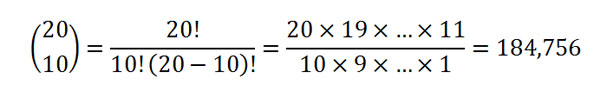
While this is a big number, consider that increasing the size of the original catalog from 20 to just 100 years yields a total of about 17,310,000,000,000 possible combinations of 10-sample extractions. AIR has an even more daunting task—to extract 10,000 simulated years of activity out of 100,000. The number of combinations in this case can basically be considered infinite, for all practical purposes. Thus, the first complicating factor in applying this concept to an actual model is the size of the catalogs and the immense number of possible solutions.

A second consideration is that during the catalog extraction process, the EP curves of different regions need to be optimized separately but simultaneously. In other words, modeled losses must be stable between the different sized catalogs throughout the exceedance probability curve, not only at an aggregate level but also for individual regions.

Suppose that we add an additional region to our example above so that each year of simulated activity is associated with two losses, one for each region (indicated by the dotted lines in Figure 4). What is the impact of applying the previous extraction solution to losses in the second region? The left panel in Figure 4 shows the new EP curve for each region. As before, the error for Region 1 is zero, but there are mismatches in the EP curve for Region 2 at the 3/10 and 7/10 probability points (as shown by the red arrows). Is there a solution that provides a faithful representation of the original catalog for both regions simultaneously? By exchanging sample 9 from the 20-year catalog for sample 17, the right panel shows a superior solution that reduces the error in regions to zero.

While we were able to find a solution in this example that minimizes the chosen error metric to zero in two regions simultaneously, this may not always be possible. As a matter of fact, it often isn't. As before, the size of the catalog plays a role, but in addition, AIR catalogs are optimized simultaneously for many more than two regions. For example, the 10,000-year catalog for the AIR Earthquake Model for Central America was optimized to eight regions (the countries of Belize, El Salvador, Guatemala, Costa Rica, Nicaragua, Honduras and Panama, in addition to the entire Central America model domain).

Optimized Earthquake Catalogs: The Value Proposition

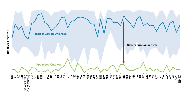
To represent the seismic behavior of regions that exhibit low seismicity (such as Northern Europe and the Central United States), AIR begins with a sample of 1,000,000 years of simulated earthquake activity from which the 100,000-year catalog is extracted. For the past decade, AIR has been developing smarter ways extract our 100,000- and 10,000-year catalogs. For example, for the 2009 release of the AIR Earthquake Model for the United States, the geography of the continental U.S. was divided into 52 zones: one for each of the 48 continental states, one additional zone for California (which was split into Northern and Southern CA), one for the District of Columbia, one for the New Madrid Seismic Zone, and a large zone that included the entire domain. Ten different random extractions of 10,000 years of simulated activity were taken from the 100,000-year catalog, and the sampling error of these extractions, in terms of losses to the total industry exposures were compared to the sampling error of AIR's the catalog built using optimization techniques.

Figure 5 shows the error associated with the random extractions (shaded area) by zone (on the horizontal axis), along with the average error among these samples (indicated by the blue line). The optimized sample (shown in green) shows a drastic reduction in error of nearly 90% on average in the 52 EP curves considered.

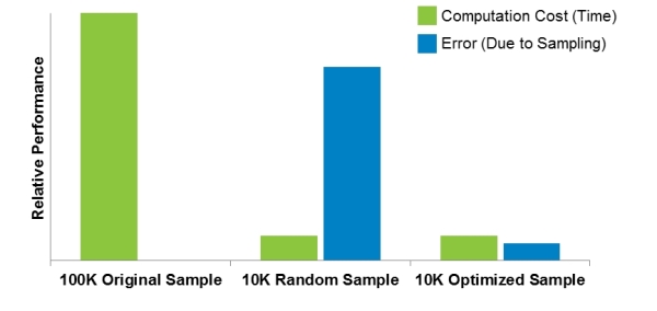
What does this mean in terms of value added by AIR's optimized catalogs? It is clear that a larger sample will always be preferable for representing stochastic processes like seismic behavior. The issue becomes assessing the trade-offs between minimizing error and minimizing computation time (which translates directly into business cost). Figure 6 shows the comparison between the large 100,000-year catalog, a randomly drawn 10,000-year sample, and an optimized 10,000-year sample in terms of computation time and sampling error (relative to the 100,000-year catalog).

A 10,000-year sample will run in approximately a tenth the time of a 100,000-year sample, meaning both the random and optimized samples yield a 90% benefit in this regard. However, the error in the random extraction is quite significant, compared with a small trade-off in accuracy in the optimized sample.

A further consideration is that the event catalog should not only give a good representation of potential losses, but also a good representation of seismic behavior in general. Earthquake models leverage several metrics that describe seismic activity across a region, which also need to be maintained as much as possible across event catalogs of different lengths. This includes Gutenberg-Richter distributions, which govern the relationship between earthquake magnitude and frequency within each seismic zone, as well as expected ground motion intensity at critical geographic locations where high concentrations of exposures are accumulated.

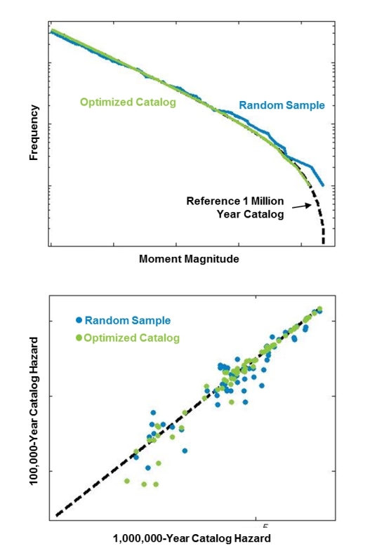
The flexibility of the optimization process (see inset) allows multiple criteria, in addition to loss, to be considered simultaneously. Figure 7 shows the impact of optimizing both magnitude-frequency distributions (top) and ground motion levels (bottom) for the 100,000-year catalog. The plot on the top shows that the optimized 100K catalog provides a much more faithful representation of the recurrence of events than the randomly extracted catalog. Similarly, the plot on the bottom shows the agreement between the 100K sample and the reference 1M catalog. The metrics on the axes represent the intensity of ground motion in the respective catalogs. A high degree of agreement is expressed by the dots falling close to the diagonal of the plot. The optimized sample shows significantly less scatter than the randomly extracted sample. In addition, keep in mind that the loss metrics and frequency metrics are optimized simultaneously, offering a much higher overall statistical fidelity in the extracted catalog.

How Does the AIR Catalog Optimization Technique Work?

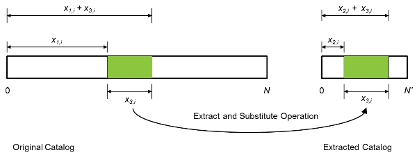
To extract a 10,000-year catalog from the full 100,000-year catalog, AIR uses a sophisticated optimization algorithm that is based on a search, extract, and substitute process (illustrated in Figure 8). From a large catalog of N years of simulated catastrophe activity, we start with a basic extraction that includes N' years from the larger sample (this first iteration can be as simple as the first N' years of the N-year catalog). The extract and substitute procedure then inserts a block of years from the original sample into the smaller catalog. This operation is defined using three variables for each iteration i of the process: x_1,i to determine the year in the original sample from which to begin the extraction; x_2,i, to determine the year in the smaller catalog from which to begin the substitution, and x₃,_i to determine the length of the extracted block.

Using a heuristic search technique, thousands of alternative extractions are constructed and candidate substitutions are repeatedly checked. The optimization process uses an objective function to measure the quality of the extracted sample. The function, which can take several objectives into consideration, has the following basic form:

f = (w₁f₁ + w₂f₂ + ... + w_kf_k) → min

where each component f_k represents a quality measure of the extracted sample, often an error metric that evaluates how closely the statistics of the extracted catalog match those of the original catalog. In AIR's earthquake models, these error metrics address the exceedance probability curves for each region of interest, the seismicity in each defined source zone, and the distribution of expected ground motions. These error metrics are each weighted with a coefficient wk and the goal is to minimize the total error function f.

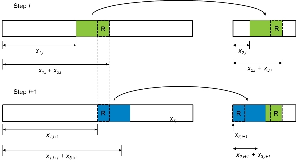
Note that the extraction and substitution algorithm, thus defined, may extract repeated samples from the original catalog, which would lead to the undesirable outcome of repeated years in the extracted catalog. Figure 9 shows two successive iterations of the process that result in a block of sample years being inserted twice (denoted with "R" in the figure).

AIR uses a strong penalty function that rejects catalog insertions that lead to duplicate years in the optimized catalog. The penalty function can take various forms, but it can be as simple as multiplying the error function by the number of repeated samples R:

f = (w₁f₁ + w₂f₂ + ... + w_kf_k) × R → min

AIR's smart search algorithms progressively sculpt the extracted catalog in such a way that its statistical properties end up accurately reflecting those of the larger catalog in as much as it is mathematically possible.

Conclusions

There is great benefit in using large samples of simulated catastrophic activity in risk models. However, there are very real business implications of doing so, including unreasonably long model run times that leave little time for decision making. For this reason, AIR routinely produces smaller samples of simulated catastrophic activity to help clients streamline their day-to-day risk management operations. Restricting the size of the sample, however, has the potential to distort the statistics for very rare events because of the effects of sampling variability that have been discussed. AIR has addressed this challenge head-on by developing sophisticated catalog extraction algorithms that minimize this distortion.

The flexibility and versatility of the catalog optimization process allows us to include multiple constraints in the sample extraction algorithm, such as maintaining magnitude-frequency, ground motion, and loss distributions in multiple seismic zones. We have achieved the construction of optimized catalogs that offer companies an almost tenfold improvement in computation performance without severely compromising accuracy, reducing statistical distortion by nearly 90% compared to random extractions. This gives companies the choice of using smaller samples with the knowledge that the overall view of seismic risk is consistent across catalogs of different sizes.